
The Format and Structure of Digital Data
Contents
6. The Format and Structure of Digital Data#
Note
This chapter authored by Todd M. Gureckis and Kelsey Moty and is released under the license for this book.
6.1. Video Lecture#
This video provides an complementary overview of this chapter. There are things mentioned in the chapter not mentioned in the video and vice versa. Together they give an overview of this unit so please read and watch.
6.2. How to think about data and organize it#
Data is an important concept in science. The first step is we measure something. In a previous chapter we discuss issues in measurement including different types of scales, units, etc… However the main thing is that data is born when a number is assigned to some observation we make. Here is a lonely single number which maybe measures something:

Things get more interesting when we make multiple observations and so we have many data. In order to do anything with more than one number though we start running into the question of how to organize things. How do we keep track of which number was collected first, second or third for instance? If we have just a big jumble of numbers we can easily get lost.
Before we get too many numbers we need to start thinking abstractly about organzing our measurements into some type of collection. In our previous chapter on the basics of Python we discussed the concept of collections. Collections are things in the native Python language space that organize multiple numbers, string, or even other collections. This included lists (which organize things in some order), dictionaries (which do not preseve order but allow “looking up” the value of a number by a special address known as a key), or sets (which are unordered collections of things useful for counting, and performing set operations like union, etc…).
For instance if we measured a number repeatedly in time a list might be a useful way to organize them:

Lets imagine the numbers above represent some measurement on a person on three different days (monday, tuesday, wednesday). It might be their blood pressure or temperature. Learning a lot about one person is nice and fits cleanly into a list. However, more often it gets more complex. What we if instead have multiple people we are recording information from and so the data starts looking two dimensional. There is maybe 3 people in the study and each has 3 measurements. In that case we might then organize the data as a list of lists (or a matrix):
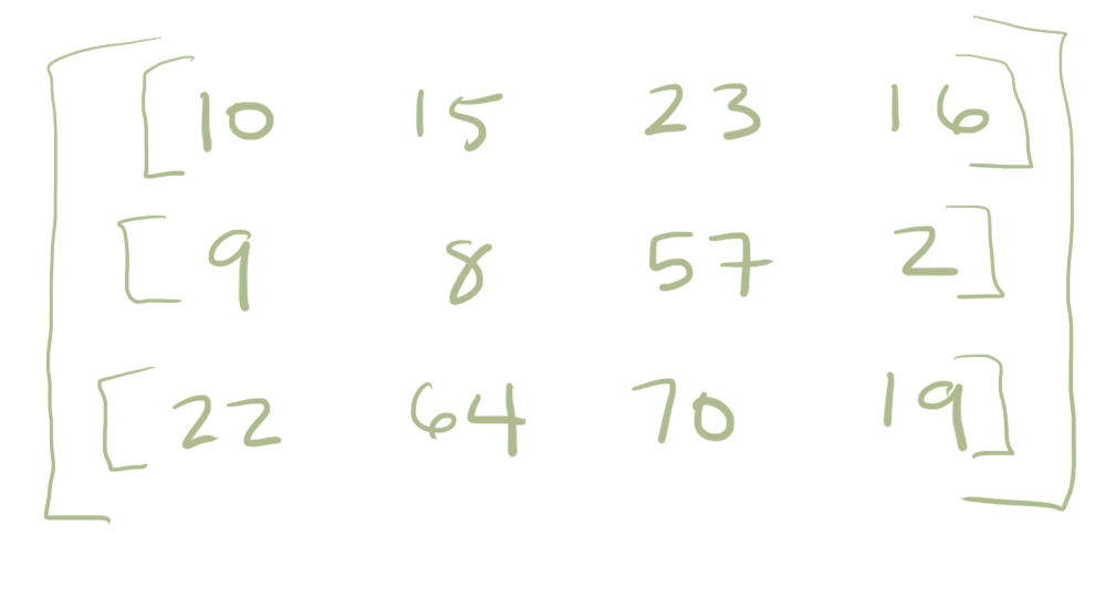
Although a matrix is a nice way to organize multiple observations made on multiple people it can get a little bit confusing. Are the rows or the columns the subjects in the example above? You have to remember to write that down otherwise you could easily get confused. What is this data? What does it describe? For this reason we might look beyond standard Python collections to more complex structures.
For example, you are all likely familiar with the concept of a spreadsheet (e.g., Microsoft Excel or Google Sheets). These are nicer than matricies because they have named rows and columns and so just by looking at the structure of the spreadsheet you can often learn more about the structure of the data. Columns names are sometimes known as metadata because they are data themselves that describe other data.
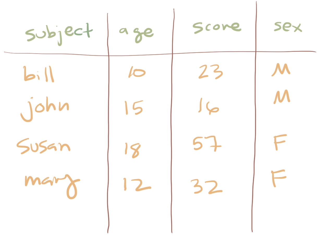
This is much nicer because the columns names help us remember what each measurement records and also what is contained in the rows.
The two dimensional structure of a spreadsheet is generally the most complex types of data that we will deal with. However, just so you are aware, as data gets really big it can make sense to take other organizational approaches. For instance, a website that had millions of users reviewing movies might not want to make a long spreadsheet recording each user and the rating they gave and the movie the rating was about. Stop and think for a moment how you could do that in a spreadsheet. Perhaps you could make each row a user and each column a movie. However, as you know Netflix and other sites have hundred of thousands of TV shows and movies and so the data would be really unweildy. Also most of the data would be “missing” because people only provide a rating for a small subset of the total number of movies. As a result, big websites adopt alternative ways of organizating data including the use of what are known as relational databases.
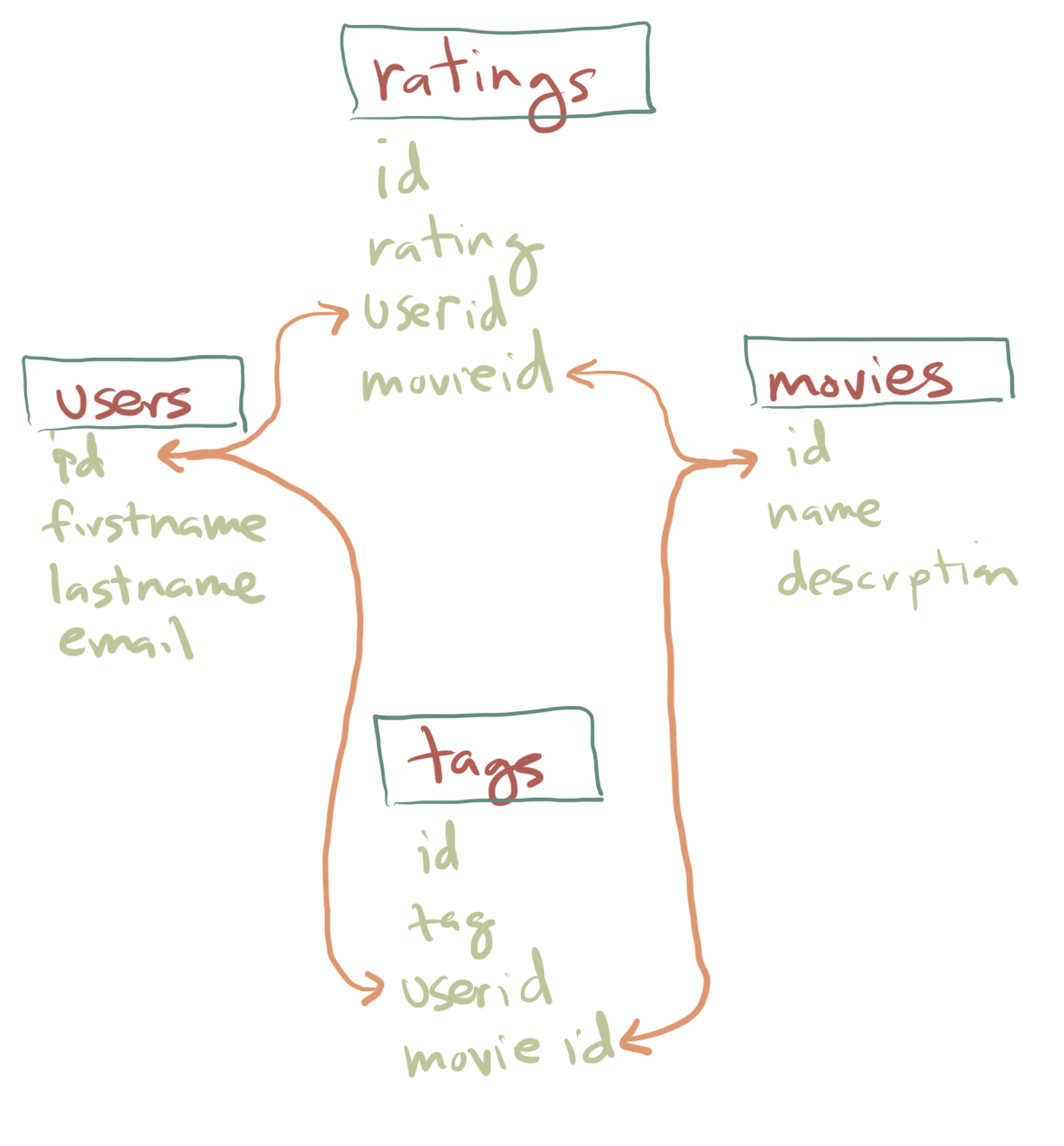
Relational databases are made up of multiple spreadsheets (effectively) where each one represents only a smaller piece of the data. In the figure above the green words are columns of a smaller spreadsheet. This database is thus organized into four separate spreadsheets (or “tables”). For instance the ratings table has an unique id number (i.e. row number) and then the rating a person gave, a user id of who gave it, and a movie id for which movie it was about. Separately there is a movies table which had its own id (unique id for each movie), the title or name of the movie, and a description/summary of the movie. The orange lines reflect links where the value in one columns of one table connects with or refers to the entries of another one. This can be a much more efficient way to organize the data.
The main point this example brings forward is that the way you organize your data is something you really have to think about and plan to begin with. I’ve found that this topic actually is intuitively interesting to many students. The reason is that we love organizing our homes and offices. It feels great. When it comes to data taking the same mentality - the “fresh” feeling of being organized, is really key to making good scientific analyses that do not have bugs. Problems with data organization can even be deadly (How not to kill people with spreadsheets). If you get really interested in organizing data, there are entire books [Glu13] and fields of study about how to best organize data (e.g., library and information sciences). The choices you make in how to organize your data at one point in time really influence how easy it can be to do certain analyses later. More on this later.
6.3. Common file formats for data#
Data often come in files with particular formatted structure. This formatted structure makes it easier for computer programs to read in the data and manipulate it. In this section we will go over a couple of the common data formats you might encounter in traditional psychological research.
6.3.1. Excel Workbooks (.xls, .xslx files)#
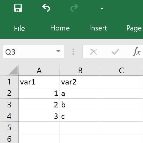
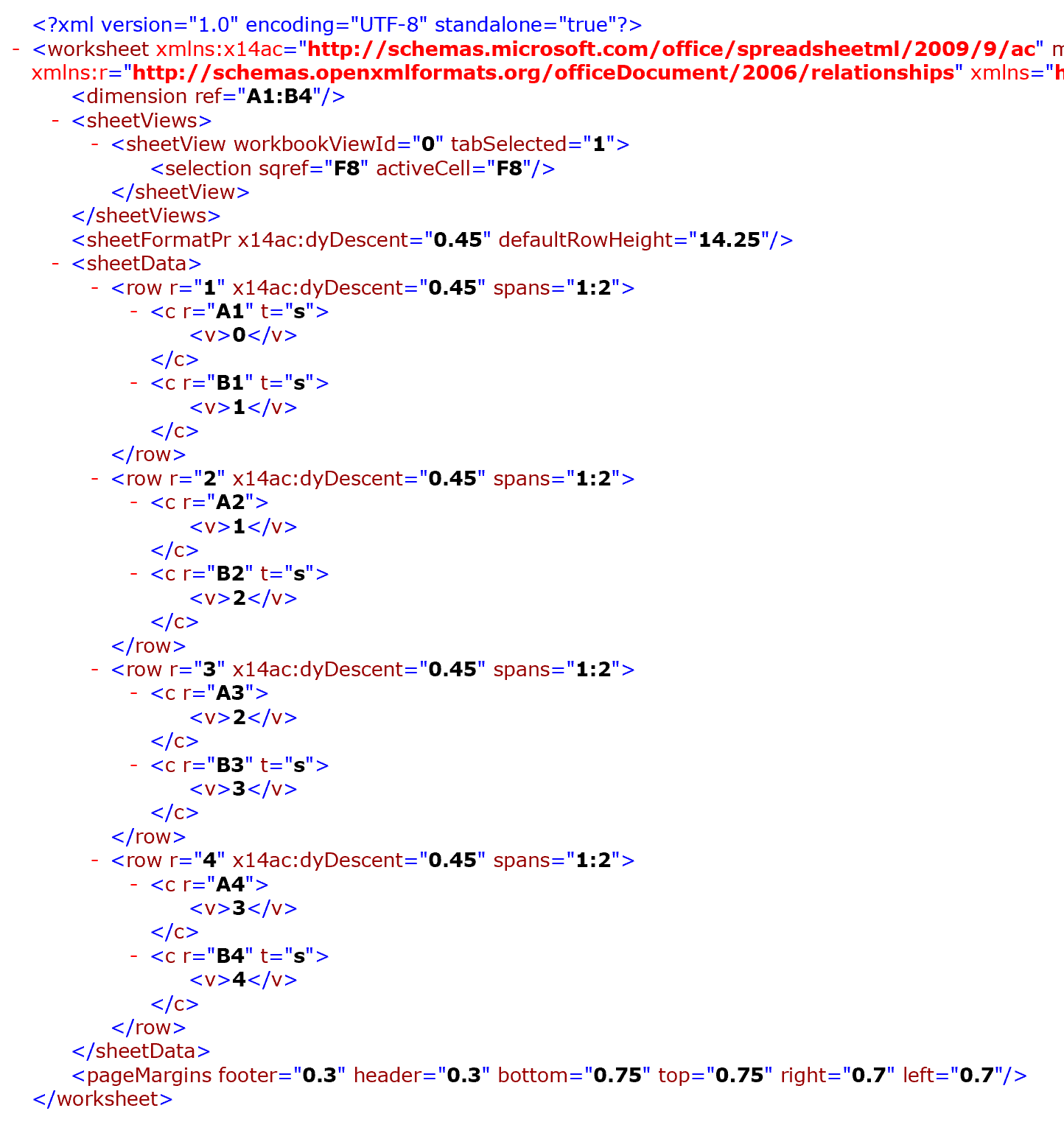
XLSX file format (or XLS in older versions of Excel) is the default file format used in Excel. Under the hood, Excel Workbooks are built using a highly structured markup language called Extensible Markup Language (XML). Essentially what this means is while you are using Excel’s graphic interface to edit your data, XML is adding a bunch of tags behind the scenes to the XLSX file so it knows how to properly format the data each time you open it up. All of these tags in XML are what allow you to change font colors and sizes, add graphs and images, and use formulas.
This is what you see when you when you use Excel:
And this is what the exact same Workbook looks like behind the scenes:
But this complexity can also make it difficult to use XLSX files with any other software or programming language that isn’t Excel. For one, not all programs can open XLSX files, so these data files can make your data inaccessible to other people. Two, all of this special formatting can sometimes lead to problems when you read in data from XLSX files (e.g., converting variables to weird formats). To avoid issues like these, it is preferable to store your data using plain-text formats (such as CSV and TSV files).
6.3.2. Comma-separated Values (.csv files)#
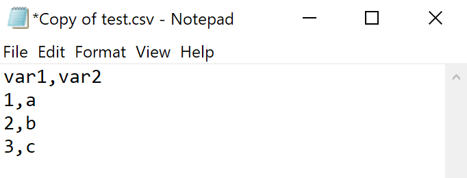
CSV, or Comma-separated value files, on the other hand, are written using a plain-text format. No special tags, just text. The only formatting in CSV files are the commas used to delimit different values for columns and new lines to indicate rows. You can see this if you open up a CSV file using Notepad (or other text editors).
Here’s the same dataset as before but now as a CSV file:
This means that what you can store within a CSV file is quite limited (no images or special formatting, for example). But it also means that this kind of file is great for storing and sharing data. CSV files can be opened by any software, making it accessible to others. Given that CSV files inherently have no formatting, some of the issues that come with using XLSX files never arise.
6.3.3. Tab-separated Values (.tsv files)#
TSV files are very similar to CSV files, except that instead of using a comma to delimit between values in a dataset, it uses tabs (a special type of spacing, the same type you get when you hit the tab key on your computer).
See also
It is a little bit beyond the scope of our class, but another file format you might encounter is referred to as JSON which stands for Javascript Object Notation (JSON). JSON is similar to a python dictionary and is stored in a plain text file like a CSV. However, JSON is somewhat more flexible than the two-dimensional structure of a spreadsheet. Often one analysis step is to convert JSON into a 2D spreadsheet-type structure. Here is a helpful guide to JSON in python.
6.4. Exporting from spreadsheet programs#
6.4.1. Google Sheets#
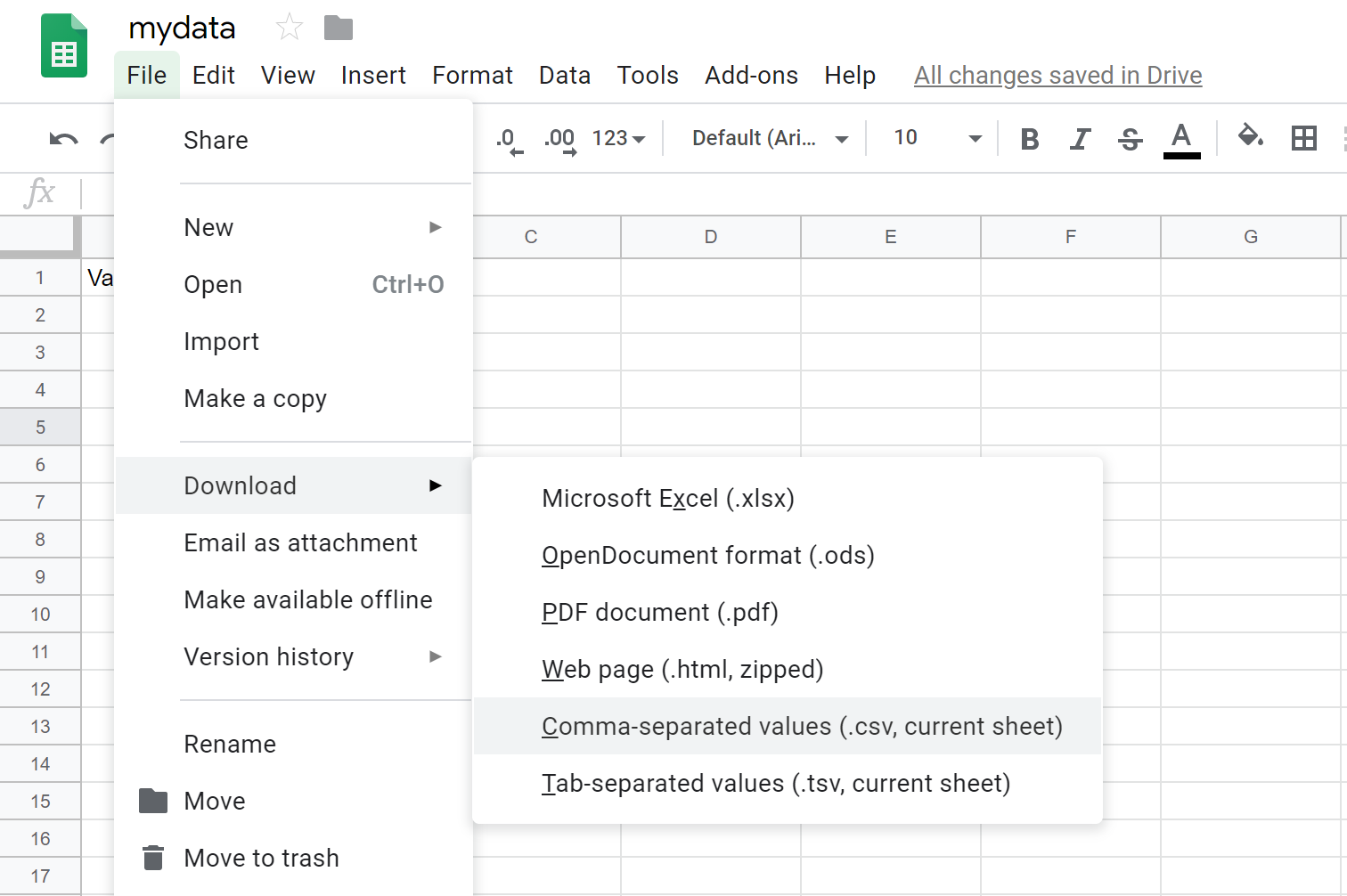
To export a .csv file from Google Sheets, you click on File > Download > Comma-separated values (.csv).
If you created a Google Sheet with multiple sheets, you will have to save each individual sheet as a .csv file because .csv files do not support multiple sheets. To do this, you will have to click on each sheet and go through the save process for each sheet.
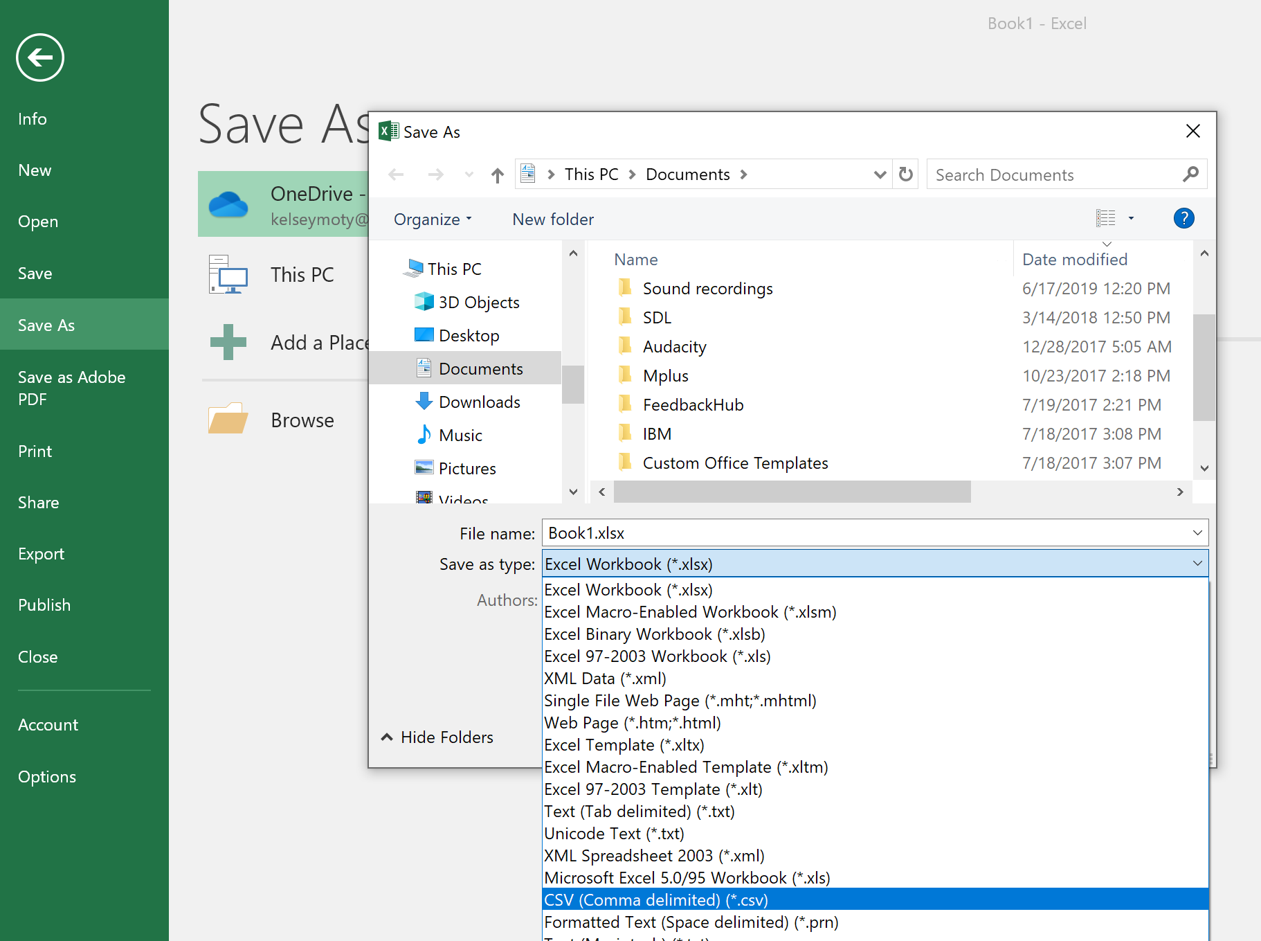
6.4.2. Excel#
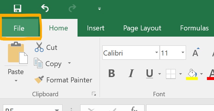
To create a .csv file from Excel, click on File (found on the top left of the menu bar).
A new menu will appear. From there, select “Save as” and then choose where on your computer you want to save the file. A pop-up window will open up, and from there, you can choose what to name the file and what kind of file type to save it as. To save it as a will there will be a dropdown menu where you can select which kind of file type you would like to save the file as (labeled “Save as type”).
6.5. Uploading csv files to JupyterHub#
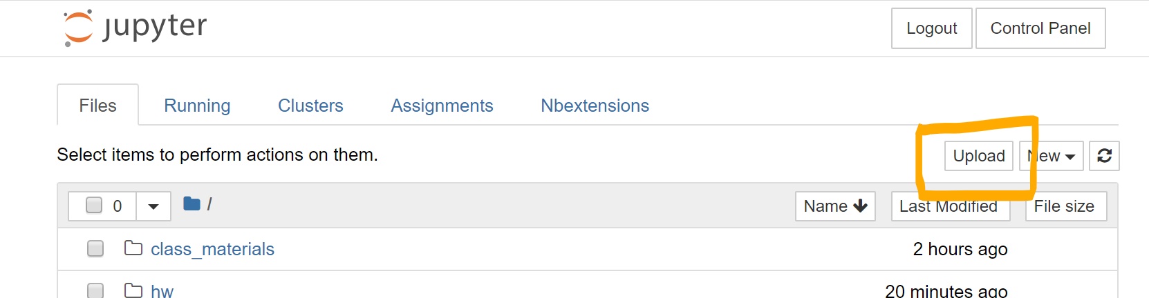
Many of the datasets you will be working with this semester will already be available for you to use on JupyterHub. However, if you want to work with your own datasets, you will need to upload them yourselves to the cluster.
To do that, go to the “Files” tab on JupyterHub and use the “Upload” button.
6.6. The Pandas library and the concept of a dataframe API#

Throughout this class there are several libraries (i.e., tools which extend the capabilities of the core Python language) which we will use a lot. One of those is Pandas. Pandas is a open-source project for Python that provides a data analysis and manipulation tool. Pandas gives you a way to interact with a dataset organized like a spreadsheet (meaning columns and rows which are possibly named or labeled with meta data) in order to perform sophisticated data analyses. Pandas is really the “backbone” of the Python data science and modeling environment. Pandas could be thought of as a langauge (or API) for unlocking tabular data. If you want to become better at data analysis with Python there is no single package I can think of that is worth more of your time learning.
Although there is no required book for this class, “Learning the Pandas Library: Python Tools for Data Munging, Analysis and Visualization” by Matt Harrison [Har16] is highly recommended both because it is short and to the point but also because it explains key Pandas concepts very clearly. In addition, the Pandas project includes a very helpful user guide which explains many of the key concepts.
Pandas can be confusing at first!
I was aware of Pandas for several years and never really “understood it.” However, when it clicked it opened a universe of data analysis to me. It takes some patience in part because data manipulation is a very complex topic at least at the conceptual level.
The organization of this guide is not to give a complete description of everything in Pandas but to kind of give you a sense of how you use Pandas (with code) to do the types of tasks you typically would do in a spreadsheet like Excel or Google Sheets. In addition, we show a few of the key features of Pandas that are not that easy to do in Excel which are very useful for behavioral data analysis.
The first step of understanding Pandas is to load it:
import numpy as np
import pandas as pd
The two code lines above are the typical way to load in the Pandas library. Numpy is a related library that Pandas is built on top of (it really is like a Russian doll where one project enables the next!). Tradionally, pandas is imported ‘as’ pd and numpy ‘as’ np. This means that when you are reading code online if you see pd.somefunction() you can probably assume that the function is part of the pandas library because the function begins with the pd. syntax.
6.7. Reading data (e.g., csvs) into Python using Pandas#
Before getting further with Pandas it helps to first understand how to read some data into a dataframe object or how to create a dataframe from scratch. Usually you are reading data in from some other file (e.g., a CSV file) and “loading” it into Pandas. Pandas has many different ways for reading in different file types. Here, we will use pd.read_csv() because we will mostly be working with .csv files in this class.
When reading in your .csv file, there are two things you absolutely have to do:
First, you need to store the data into a variable. Otherwise, you won’t be able to work with your data. Here, we called the dataframe “df” but you can name it whatever you want.
# incorrect: won't store your data
pd.read_csv('salary.csv')

# correct: creates a dataframe called df that you can work with
df = pd.read_csv('salary.csv')
Second, you need to tell pd.read_csv where the file you are trying to import is located. The path can point to a file located in a folder in your local enviroment (e.g., on your computer, on JupyterHub) or to a file available online.
To point to a file available online, you’ll put the link to the file.
df = pd.read_csv('http://gureckislab.org/courses/fall19/labincp/data/salary.csv')
If you are pointing to a file on JupyterHub (or to a file on your computer, if you had Python downloaded on your computer), you’ll need to specify the path to the file. If the .csv file and your notebook are in the same folder, you only have to put the name of the file.
df = pd.read_csv('salary.csv')
If the file is located in a different folder than the notebook you are working with, you will have to specify which folder(s) that the computer needs to look at to find it.
df = pd.read_csv('folder1/folder2/salary.csv')
Sometimes, your .csv file might be saved in a folder that’s not in the same folder as your notebook. For example, say you have a folder called “project”. And in that the folder, there was a folder called “code” that contained your notebooks/python code, as well as a folder called “data” that contained your data (.csv) files. To import your .csv file, you need to use .. to tell the your computer go up one folder in your directory (get out of the “code” folder) in order for it to find the “data” folder.
df = pd.read_csv('../data/salary.csv')
By default, pd.read_csv assumes that file uses commas to differentiate between different entries in the file. But you can also explicitly tell pd.read_csv that you want to use commas as the delimiter.
df = pd.read_csv('salary.csv', sep = ",")
pd.read_csv also assumes by default that the first row in your .csv files lists the names for each column of data (the column headers). You can explicitly tell pd.read_csv to do this by writing:
df = pd.read_csv('salary.csv', sep = ",", header = 'infer')
Sometimes, datasets may have multiple headers. (e.g., both the first and second rows of the dataset list column names). pd.read_csv allows you to keep both rows as headers by modifying the header argument with a list of integers. Remember that 0 actually means the first row.
df = pd.read_csv('salary.csv', sep = ",", header = [0,1])
When creating your own datasets, it’s generally best practice to give your columns headers, so that’s it easier for people looking at your data (including yourself!) to know what’s in the dataset. However, you may occassionally come across datasets that do not have headers. To tell pd.read_csv there’s no header to import, set header to “None”:
df = pd.read_csv('salary.csv', sep = ",", header = None)
:::{warning} When creating your own dataset, refrain from using characters like space or period (.) in the column names. This will make things easier for you down the line when using Pandas for statistical modeling. :::
6.8. Viewing the data in a dataframe#
So now we have loaded a dataset into a variable called df. Now we might like to look at the data to check it was properly read in and also to learn more about the structure of this dataset. Perhaps the simplest method is simply to type the name of the dataframe variable by itself in a code cell:
df = pd.read_csv('http://gureckislab.org/courses/fall19/labincp/data/salary.csv')
df
| salary | gender | departm | years | age | publications | |
|---|---|---|---|---|---|---|
| 0 | 86285 | 0 | bio | 26.0 | 64.0 | 72 |
| 1 | 77125 | 0 | bio | 28.0 | 58.0 | 43 |
| 2 | 71922 | 0 | bio | 10.0 | 38.0 | 23 |
| 3 | 70499 | 0 | bio | 16.0 | 46.0 | 64 |
| 4 | 66624 | 0 | bio | 11.0 | 41.0 | 23 |
| ... | ... | ... | ... | ... | ... | ... |
| 72 | 53662 | 1 | neuro | 1.0 | 31.0 | 3 |
| 73 | 57185 | 1 | stat | 9.0 | 39.0 | 7 |
| 74 | 52254 | 1 | stat | 2.0 | 32.0 | 9 |
| 75 | 61885 | 1 | math | 23.0 | 60.0 | 9 |
| 76 | 49542 | 1 | math | 3.0 | 33.0 | 5 |
77 rows × 6 columns
This outputs a “table” view of the dataframe showing the column names, and several of the rows of the dataset. It doesn’t show you all of the data at once because in many large files this would be too much to make sense of.
You can also specifically request the first several rows of the dataframe:
df.head()
| salary | gender | departm | years | age | publications | |
|---|---|---|---|---|---|---|
| 0 | 86285 | 0 | bio | 26.0 | 64.0 | 72 |
| 1 | 77125 | 0 | bio | 28.0 | 58.0 | 43 |
| 2 | 71922 | 0 | bio | 10.0 | 38.0 | 23 |
| 3 | 70499 | 0 | bio | 16.0 | 46.0 | 64 |
| 4 | 66624 | 0 | bio | 11.0 | 41.0 | 23 |
or the last several rows:
df.tail()
| salary | gender | departm | years | age | publications | |
|---|---|---|---|---|---|---|
| 72 | 53662 | 1 | neuro | 1.0 | 31.0 | 3 |
| 73 | 57185 | 1 | stat | 9.0 | 39.0 | 7 |
| 74 | 52254 | 1 | stat | 2.0 | 32.0 | 9 |
| 75 | 61885 | 1 | math | 23.0 | 60.0 | 9 |
| 76 | 49542 | 1 | math | 3.0 | 33.0 | 5 |
The “head” of the dataframe is the top. The “tail” of the dataframe is the bottom.
We can also access individual rows and columns of a data frame.
6.8.1. Accessing individual columns#
To access a single column you can index it like a dictionary in Python using the column name as a key:
df['salary']
0     86285
1     77125
2     71922
3     70499
4     66624
      ...
72    53662
73    57185
74    52254
75    61885
76    49542
Name: salary, Length: 77, dtype: int64
df['age']
0     64.0
1     58.0
2     38.0
3     46.0
4     41.0
      ...
72    31.0
73    39.0
74    32.0
75    60.0
76    33.0
Name: age, Length: 77, dtype: float64
Another allowed syntax is to use the name of the dataframe variable and a .columnname. For instance:
df.salary
0     86285
1     77125
2     71922
3     70499
4     66624
      ...
72    53662
73    57185
74    52254
75    61885
76    49542
Name: salary, Length: 77, dtype: int64
However the dictionary key-lookup method is preferred because it is possible that the name of a column is the same as a dataframe method (see below) and that causes Python to get confused.
:::{seealso} When we learn about visualizing data, describing data, and linear regression you will see how the column struture of dataframes becomes very powerful. :::
6.8.2. Accessing individal rows#
Since the Python bracket notation is use to lookup columns, a special command is needed to access rows. The best way to look up a single row is to use .iloc[] where you pass the integer row number you want to access (zero indexed). So to get the first row you type:
df.iloc[0]
salary          86285
gender              0
departm           bio
years              26
age                64
publications       72
Name: 0, dtype: object
Here is the 5th row:
df.iloc[4]
salary          66624
gender              0
departm           bio
years              11
age                41
publications       23
Name: 4, dtype: object
or counting three backwards from the end:
df.iloc[-3]
salary          52254
gender              1
departm          stat
years               2
age                32
publications        9
Name: 74, dtype: object
6.8.3. Indexes and Columns#
Also note that there are two special elements of a normal dataframe called the column index and the row index (or just index). The row index is the column on the left that has no name but seems like a counter of the rows (e.g., 72, 73, 74, …). The row index is useful in Pandas dataframes for looking things up by row. Although you can index a row by counting (access the fifth row for instance), the index can be made on arbitrary types of data including strings, etc… You don’t need to know a ton about indexes to use Pandas typically but every once in a while they come up so it is useful to know the special nature of the index column.
df.index
RangeIndex(start=0, stop=77, step=1)
df.columns
Index(['salary', 'gender', 'departm', 'years', 'age', 'publications'], dtype='object')
The above code shows how to find the row index and column index.
You can change the row index to another column:
df.set_index('departm')
| salary | gender | years | age | publications | |
|---|---|---|---|---|---|
| departm | |||||
| bio | 86285 | 0 | 26.0 | 64.0 | 72 |
| bio | 77125 | 0 | 28.0 | 58.0 | 43 |
| bio | 71922 | 0 | 10.0 | 38.0 | 23 |
| bio | 70499 | 0 | 16.0 | 46.0 | 64 |
| bio | 66624 | 0 | 11.0 | 41.0 | 23 |
| ... | ... | ... | ... | ... | ... |
| neuro | 53662 | 1 | 1.0 | 31.0 | 3 |
| stat | 57185 | 1 | 9.0 | 39.0 | 7 |
| stat | 52254 | 1 | 2.0 | 32.0 | 9 |
| math | 61885 | 1 | 23.0 | 60.0 | 9 |
| math | 49542 | 1 | 3.0 | 33.0 | 5 |
77 rows × 5 columns
Or to reset it to a counter that count the row number use .reset_index().
df2=df.set_index('departm')
df2.reset_index()
| departm | salary | gender | years | age | publications | |
|---|---|---|---|---|---|---|
| 0 | bio | 86285 | 0 | 26.0 | 64.0 | 72 |
| 1 | bio | 77125 | 0 | 28.0 | 58.0 | 43 |
| 2 | bio | 71922 | 0 | 10.0 | 38.0 | 23 |
| 3 | bio | 70499 | 0 | 16.0 | 46.0 | 64 |
| 4 | bio | 66624 | 0 | 11.0 | 41.0 | 23 |
| ... | ... | ... | ... | ... | ... | ... |
| 72 | neuro | 53662 | 1 | 1.0 | 31.0 | 3 |
| 73 | stat | 57185 | 1 | 9.0 | 39.0 | 7 |
| 74 | stat | 52254 | 1 | 2.0 | 32.0 | 9 |
| 75 | math | 61885 | 1 | 23.0 | 60.0 | 9 |
| 76 | math | 49542 | 1 | 3.0 | 33.0 | 5 |
77 rows × 6 columns
Note the syntax we’ve used a few times here… we referenced the df variable which is the variable we created to store the data from our file. Then the .functionname() is known as a method of the data frame which is provided by pandas. For instance the .head() method prints out the first five rows of the data frame. The .tail() method prints out the last five rows of the data frame. There are many other methods available on data frames that you access by calling it using the .functionname() syntax. The next parts of this chapter explain some of the most common ones.
6.9. Adding and deleting things from a dataframe#
Sometimes after we read in a dataset we might want to add new rows or columns or delete rows and columns from a dataframe. One way to do this is to edit the original CSV file that we read in. However, there is an important principle I want to emphasize thoughout this class:
ALWAYS do everything in code
What do I mean by do everything in code? What I mean is that if you go to your data file that you got from some place and then by hand delete some of the data in Google Sheets or Excel, noone will know that you did that. There is no record of it. Once you save the file the data will be deleted and noone will know you did this. Instead if you keep your data as “raw” as possible and modify it using code, your code will document ALL of the steps you did in your analysis including the step of deleting data. “Excluding” (not DELETEing) data is sometimes justified but the important thing is we want to document all our steps honestly and truthfully when doing analysis. Using code to do every single step of an analysis helps us accomplish this.
6.9.1. Deleting rows#
To delete a row you can use the .drop() method to drop a particular item using its index value. The .drop() method is not an “in place operation” instead it returns a new dataframe with the particular rows removed.
“In place” operations
From time to time using pandas you will here about a method being described as “in place” or “not in place.” In place means that the change you are making to the dataframe is made to the dataframe variable you describe. So for instance if you have a dataframe stored in a variable named df and you call df.drop([1]) it will drop the row corresponding to the index value 1. However, if you look at df again using, for instance, df.head() you will see that it will not have changed. To save the changes with a “not in place” operation you need to store the results in a new variable. For insteance df2 = df.drop([1]) will make a copy of df, drop the row corresponding to index 1 and then store the result in df2. If drop was an “in place” operation it would have actually modified df and so you wouldn’t need to store the result in a new variable.
Here is how to use it. Suppose we have the salary dataframe from above:
df.head()
| salary | gender | departm | years | age | publications | |
|---|---|---|---|---|---|---|
| 0 | 86285 | 0 | bio | 26.0 | 64.0 | 72 |
| 1 | 77125 | 0 | bio | 28.0 | 58.0 | 43 |
| 2 | 71922 | 0 | bio | 10.0 | 38.0 | 23 |
| 3 | 70499 | 0 | bio | 16.0 | 46.0 | 64 |
| 4 | 66624 | 0 | bio | 11.0 | 41.0 | 23 |
If we want to delete the first we can drop it using the index it has, in this case 0:
df2=df.drop([0])
df2.head()
| salary | gender | departm | years | age | publications | |
|---|---|---|---|---|---|---|
| 1 | 77125 | 0 | bio | 28.0 | 58.0 | 43 |
| 2 | 71922 | 0 | bio | 10.0 | 38.0 | 23 |
| 3 | 70499 | 0 | bio | 16.0 | 46.0 | 64 |
| 4 | 66624 | 0 | bio | 11.0 | 41.0 | 23 |
| 5 | 64451 | 0 | bio | 23.0 | 60.0 | 44 |
Notice how I “saved” the modified dataframe into a new variable called df2 using the equals sign. Then if we call the .head() method on df2 we can see that the first row has been removed. df, the original dataframe variable, remains unchanged.
You can also remove multiple rows by their index value at once:
df.drop([0,2,4,6]).head()
| salary | gender | departm | years | age | publications | |
|---|---|---|---|---|---|---|
| 1 | 77125 | 0 | bio | 28.0 | 58.0 | 43 |
| 3 | 70499 | 0 | bio | 16.0 | 46.0 | 64 |
| 5 | 64451 | 0 | bio | 23.0 | 60.0 | 44 |
| 7 | 59344 | 0 | bio | 5.0 | 40.0 | 11 |
| 8 | 58560 | 0 | bio | 8.0 | 38.0 | 8 |
Here I dropped the rows with index 0,2,4,6, and also show an example of chaining dataframe methods.
Chaining methods
Dataframes in pandas a what is known as an object-oriented structure. This means that most the functionality of a dataframe is tied to the variables themselves. That is why in the previous examples we called df.method() like df.drop() instead of pd.drop() (calling from the base pandas library). Given this, most pandas methods either return themselves or a copy of the dataframe that has been altered. Thus you can “chain” operations and methods together to make the code more concise. Chaining means calling multiple methods in a row on a single line of code. df.drop([0,2,4,6]).head() calls the drop() method on the dataframe and then called the head() method on the resulting modified data frame. This means you don’t have to store every intermediate step of your data manipulation into a new variable.
6.9.2. Deleting columns#
To delete a column instead of a row you can also use the .drop() method, using an additional argument that refers to the “axis” you are dropping from.
df.head()
| salary | gender | departm | years | age | publications | |
|---|---|---|---|---|---|---|
| 0 | 86285 | 0 | bio | 26.0 | 64.0 | 72 |
| 1 | 77125 | 0 | bio | 28.0 | 58.0 | 43 |
| 2 | 71922 | 0 | bio | 10.0 | 38.0 | 23 |
| 3 | 70499 | 0 | bio | 16.0 | 46.0 | 64 |
| 4 | 66624 | 0 | bio | 11.0 | 41.0 | 23 |
Here are a couple examples of dropping one or more columns by name. Note that the case of the column name must match and also you need to specific axis=1 to refer to dropping columns instead of rows.
df.drop('years',axis=1).head()
| salary | gender | departm | age | publications | |
|---|---|---|---|---|---|
| 0 | 86285 | 0 | bio | 64.0 | 72 |
| 1 | 77125 | 0 | bio | 58.0 | 43 |
| 2 | 71922 | 0 | bio | 38.0 | 23 |
| 3 | 70499 | 0 | bio | 46.0 | 64 |
| 4 | 66624 | 0 | bio | 41.0 | 23 |
df.drop(['years','age'],axis=1).head()
| salary | gender | departm | publications | |
|---|---|---|---|---|
| 0 | 86285 | 0 | bio | 72 |
| 1 | 77125 | 0 | bio | 43 |
| 2 | 71922 | 0 | bio | 23 |
| 3 | 70499 | 0 | bio | 64 |
| 4 | 66624 | 0 | bio | 23 |
6.9.3. Adding rows#
Using pandas it is best to resist the urge to add rows one at a time to a dataframe. For various reasons is this not the ideal way to use pandas 1. Instead you can combine the rows of two different dataframes into one. This might be useful in psychology for instance if each participant in your experiment had their own data file and you want to read each file into a dataframe and them combine them together to make one “uber” dataframe with all the data from your experiment.
Here’s two simple dataframes and we can combine them:
df1 = pd.DataFrame({"age": [10,27,45,23,21], "salary": [0,23000,100000,35000,60000]})
df2 = pd.DataFrame({"age": [60,70,53,56,80], "salary": [50000,23000,60000,135000,0]})

df_combined = pd.concat([df1,df2])

df_combined
| age | salary | |
|---|---|---|
| 0 | 10 | 0 |
| 1 | 27 | 23000 |
| 2 | 45 | 100000 |
| 3 | 23 | 35000 |
| 4 | 21 | 60000 |
| 0 | 60 | 50000 |
| 1 | 70 | 23000 |
| 2 | 53 | 60000 |
| 3 | 56 | 135000 |
| 4 | 80 | 0 |
This only works because they have the same columns. If they have different columns then the missing entries of either are filled in with NaN which is the code for “missing values” in pandas.
df1 = pd.DataFrame({"age": [10,27,45,23,21], "salary": [0,23000,100000,35000,60000]})
df2 = pd.DataFrame({"age": [60,70,53,56,80], "height": [5.2,6.0,5.7,3.4,4.6]})

df_combined = pd.concat([df1,df2])

df_combined
| age | salary | height | |
|---|---|---|---|
| 0 | 10 | 0.0 | NaN |
| 1 | 27 | 23000.0 | NaN |
| 2 | 45 | 100000.0 | NaN |
| 3 | 23 | 35000.0 | NaN |
| 4 | 21 | 60000.0 | NaN |
| 0 | 60 | NaN | 5.2 |
| 1 | 70 | NaN | 6.0 |
| 2 | 53 | NaN | 5.7 |
| 3 | 56 | NaN | 3.4 |
| 4 | 80 | NaN | 4.6 |
We will talk about dealing with “missing” values shortly but basically missing values in pandas allows for incomplete rows: you might have have information about every single field of a row and so you can uses NaN (stands for Not-a-number in computer speak) to represent missing values.
6.9.4. Adding columns#
As we have considered adding rows, now let’s consider adding columns. This is actually pretty easy. You just assign some values to a new columns name. First we will create a data frame with two random columns:
df = pd.DataFrame({"col_1": np.random.rand(10), "col_2": np.random.rand(10)})
df
| col_1 | col_2 | |
|---|---|---|
| 0 | 0.016417 | 0.555351 |
| 1 | 0.323619 | 0.868004 |
| 2 | 0.744349 | 0.767006 |
| 3 | 0.023376 | 0.915717 |
| 4 | 0.431546 | 0.761252 |
| 5 | 0.668849 | 0.522965 |
| 6 | 0.199476 | 0.161559 |
| 7 | 0.071968 | 0.866112 |
| 8 | 0.452259 | 0.650265 |
| 9 | 0.449017 | 0.797710 |
Now we simply assign a new column df[\'sum\'] and define it to be the sum of two columns.
df['sum'] = df['col_1']+df['col_2']
df
| col_1 | col_2 | sum | |
|---|---|---|---|
| 0 | 0.016417 | 0.555351 | 0.571768 |
| 1 | 0.323619 | 0.868004 | 1.191623 |
| 2 | 0.744349 | 0.767006 | 1.511355 |
| 3 | 0.023376 | 0.915717 | 0.939093 |
| 4 | 0.431546 | 0.761252 | 1.192798 |
| 5 | 0.668849 | 0.522965 | 1.191814 |
| 6 | 0.199476 | 0.161559 | 0.361035 |
| 7 | 0.071968 | 0.866112 | 0.938080 |
| 8 | 0.452259 | 0.650265 | 1.102524 |
| 9 | 0.449017 | 0.797710 | 1.246726 |
You can also define new columns to be a constant value:
df['constant'] = 2
df
| col_1 | col_2 | sum | constant | |
|---|---|---|---|---|
| 0 | 0.189631 | 0.014450 | 0.204081 | 2 |
| 1 | 0.455379 | 0.781008 | 1.236386 | 2 |
| 2 | 0.879715 | 0.426790 | 1.306504 | 2 |
| 3 | 0.942081 | 0.905498 | 1.847578 | 2 |
| 4 | 0.189411 | 0.631864 | 0.821275 | 2 |
| 5 | 0.813499 | 0.069108 | 0.882607 | 2 |
| 6 | 0.884211 | 0.467572 | 1.351783 | 2 |
| 7 | 0.232354 | 0.593110 | 0.825464 | 2 |
| 8 | 0.762218 | 0.176046 | 0.938265 | 2 |
| 9 | 0.872711 | 0.053765 | 0.926476 | 2 |
There are of course some limitations and technicalities here but for the most part you just name a new column and define it as above.
6.9.5. Deleting rows with missing data#
Since we are talking about adding and removing rows and columns it can also make sense to discuss removing rows with missing data. You might want to for example drop any trial from an experiment where a subject didn’t give a response before a timer deadline. In this case the column coding what the response was might be “empty” or “missing” and you would want to use the NaN value to indicate it was missing. To totally delete rows with any missing value use the dropna() function:
df = pd.DataFrame({"age": [10,27,45,23,21], "salary": [0,23000,None,35000,60000]})
df
| age | salary | |
|---|---|---|
| 0 | 10 | 0.0 |
| 1 | 27 | 23000.0 |
| 2 | 45 | NaN |
| 3 | 23 | 35000.0 |
| 4 | 21 | 60000.0 |
As you can see the salary value is missing for row with index 2 (age 45). To drop any row with a missing value:
df.dropna()
| age | salary | |
|---|---|---|
| 0 | 10 | 0.0 |
| 1 | 27 | 23000.0 |
| 3 | 23 | 35000.0 |
| 4 | 21 | 60000.0 |
There are several other tricks for dropping missing data besides this. For example, you can delete rows with only a specific column value missing, etc… However for now this should work for us.
6.9.6. Getting individual values and changing them#
Sometimes you want to just extract a single value or row from a dataframe or change a single value. The .iat method lets you pull out a single value from the data frame given the position of the index and column. The .iat method is one of the very weird parts of Pandas which has no real good explanation. Instead of the parentheses used to call normal methods, .iat and a few others use square brackets. One way to think about it is that .iat is like looking something up in a normal Python array but it also seems like a method attached to the dataframe.
df = pd.read_csv('http://gureckislab.org/courses/fall19/labincp/data/salary.csv')
df
| salary | gender | departm | years | age | publications | |
|---|---|---|---|---|---|---|
| 0 | 86285 | 0 | bio | 26.0 | 64.0 | 72 |
| 1 | 77125 | 0 | bio | 28.0 | 58.0 | 43 |
| 2 | 71922 | 0 | bio | 10.0 | 38.0 | 23 |
| 3 | 70499 | 0 | bio | 16.0 | 46.0 | 64 |
| 4 | 66624 | 0 | bio | 11.0 | 41.0 | 23 |
| ... | ... | ... | ... | ... | ... | ... |
| 72 | 53662 | 1 | neuro | 1.0 | 31.0 | 3 |
| 73 | 57185 | 1 | stat | 9.0 | 39.0 | 7 |
| 74 | 52254 | 1 | stat | 2.0 | 32.0 | 9 |
| 75 | 61885 | 1 | math | 23.0 | 60.0 | 9 |
| 76 | 49542 | 1 | math | 3.0 | 33.0 | 5 |
77 rows × 6 columns
This gets the value at row 0 column 0 which is the salary of the first person in the data frame.
df.iat[0,0]
86285
This gets the age of the person in the sixth row, fourth column.
df.iat[6,4]
53.0
A slighly more reader-friendly option is to use .at[] which is a method that lets you look things up using the names of columns.
df.at[10, 'age']
40.0
You can also use this to change the value of a particular cell.
First we see that the person in the first row has age 64.
df.head()
| salary | gender | departm | years | age | publications | |
|---|---|---|---|---|---|---|
| 0 | 86285 | 0 | bio | 26.0 | 64.0 | 72 |
| 1 | 77125 | 0 | bio | 28.0 | 58.0 | 43 |
| 2 | 71922 | 0 | bio | 10.0 | 38.0 | 23 |
| 3 | 70499 | 0 | bio | 16.0 | 46.0 | 64 |
| 4 | 66624 | 0 | bio | 11.0 | 41.0 | 23 |
Using .at[] we set it to 100.
df.at[0,'age']=100
Then when we look at the result the age has been changed in the dataframe df.
df.head()
| salary | gender | departm | years | age | publications | |
|---|---|---|---|---|---|---|
| 0 | 86285 | 0 | bio | 26.0 | 100.0 | 72 |
| 1 | 77125 | 0 | bio | 28.0 | 58.0 | 43 |
| 2 | 71922 | 0 | bio | 10.0 | 38.0 | 23 |
| 3 | 70499 | 0 | bio | 16.0 | 46.0 | 64 |
| 4 | 66624 | 0 | bio | 11.0 | 41.0 | 23 |
The way to remember this is that methods that look things up use square brackets. And if the method begins with an i (like .iat[]) it will look it up by integer index (i.e., the number of the column or row). Otherwise .at[] looks up by row (or a named index) and column name.
6.9.7. Checking the size/dimensions of your data#
One common thing you need to do is to verify the number of rows and columns in your dataframe. The .shape property can help with that.
df = pd.read_csv('http://gureckislab.org/courses/fall19/labincp/data/salary.csv')
df.shape
(77, 6)
This tells us that the dataframe contained in variable df has 77 rows and 6 columns. This is often helpful when you first read in a dataset to verify it has all the data you expected to be there!
Methods versus properties
The .shape property doesn’t include a final () unlike other methods we have learned about like .drop() which required parentheses. This reflects that size is known as a property of the dataframe while .drop() is a method. The conceptual differences can be confusing for why one is one way or the other. However, it is helpful to often think about them as the distinction between nouns and verbs in langauge. Properties (nouns) are static descriptors of a dataset such as the size of the dataset or the column names. In contrast, methods (verbs) are things that require computation or modification of the dataframe like deleting things or performing computations on columns or rows.
Ultimately the step we just covered recreate much of what you do with the graphical user interface in Excel (change cell values, add/delete rows and columns, etc…). The real power of Pandas comes from more complex things you can do with dataframes. That is what we will explore in the next section.
6.10. Things you can do with dataframes#
The main goal of getting your data into a dataframe is that enables several methods for manipulating your data in powerful ways.
6.10.1. Sorting#
Often times it can help us understand a dataset better if we can sort the rows of the dataset according to the values in one or more columns. For instance in the salary data set we have been considering it is hard to know who is the highest and lowest paid faculty. One approach would to be sort the values.
df = pd.read_csv('http://gureckislab.org/courses/fall19/labincp/data/salary.csv')
df.head()
| salary | gender | departm | years | age | publications | |
|---|---|---|---|---|---|---|
| 0 | 86285 | 0 | bio | 26.0 | 64.0 | 72 |
| 1 | 77125 | 0 | bio | 28.0 | 58.0 | 43 |
| 2 | 71922 | 0 | bio | 10.0 | 38.0 | 23 |
| 3 | 70499 | 0 | bio | 16.0 | 46.0 | 64 |
| 4 | 66624 | 0 | bio | 11.0 | 41.0 | 23 |
We can sort this dataset in ascending order with:
df.sort_values('salary')
| salary | gender | departm | years | age | publications | |
|---|---|---|---|---|---|---|
| 23 | 44687 | 0 | chem | 4.0 | 34.0 | 19 |
| 22 | 47021 | 0 | chem | 4.0 | 34.0 | 12 |
| 76 | 49542 | 1 | math | 3.0 | 33.0 | 5 |
| 53 | 51391 | 0 | stat | 5.0 | 35.0 | 8 |
| 74 | 52254 | 1 | stat | 2.0 | 32.0 | 9 |
| ... | ... | ... | ... | ... | ... | ... |
| 14 | 97630 | 0 | chem | 34.0 | 64.0 | 43 |
| 24 | 104828 | 0 | geol | NaN | 50.0 | 44 |
| 29 | 105761 | 0 | neuro | 9.0 | 39.0 | 30 |
| 41 | 106412 | 0 | stat | 23.0 | 53.0 | 29 |
| 28 | 112800 | 0 | neuro | 14.0 | 44.0 | 33 |
77 rows × 6 columns
Now we can easily see from this output at 44,687 is the lowest salary and 112,800 is the highest. sort_values() is not an inplace operation so the original dataframe is still unsorted and we have to store the sorted result in a new dataframe variable if we want to keep working with it.
df.head() # still unsorted
| salary | gender | departm | years | age | publications | |
|---|---|---|---|---|---|---|
| 0 | 86285 | 0 | bio | 26.0 | 64.0 | 72 |
| 1 | 77125 | 0 | bio | 28.0 | 58.0 | 43 |
| 2 | 71922 | 0 | bio | 10.0 | 38.0 | 23 |
| 3 | 70499 | 0 | bio | 16.0 | 46.0 | 64 |
| 4 | 66624 | 0 | bio | 11.0 | 41.0 | 23 |
We can sort the other way by adding an additional parameter:
df.sort_values('salary',ascending=False)
| salary | gender | departm | years | age | publications | |
|---|---|---|---|---|---|---|
| 28 | 112800 | 0 | neuro | 14.0 | 44.0 | 33 |
| 41 | 106412 | 0 | stat | 23.0 | 53.0 | 29 |
| 29 | 105761 | 0 | neuro | 9.0 | 39.0 | 30 |
| 24 | 104828 | 0 | geol | NaN | 50.0 | 44 |
| 14 | 97630 | 0 | chem | 34.0 | 64.0 | 43 |
| ... | ... | ... | ... | ... | ... | ... |
| 74 | 52254 | 1 | stat | 2.0 | 32.0 | 9 |
| 53 | 51391 | 0 | stat | 5.0 | 35.0 | 8 |
| 76 | 49542 | 1 | math | 3.0 | 33.0 | 5 |
| 22 | 47021 | 0 | chem | 4.0 | 34.0 | 12 |
| 23 | 44687 | 0 | chem | 4.0 | 34.0 | 19 |
77 rows × 6 columns
And if you sort by two columns it will do them in order (so the first listed column is sorted first then the second):
df.sort_values(['salary','age'])
| salary | gender | departm | years | age | publications | |
|---|---|---|---|---|---|---|
| 23 | 44687 | 0 | chem | 4.0 | 34.0 | 19 |
| 22 | 47021 | 0 | chem | 4.0 | 34.0 | 12 |
| 76 | 49542 | 1 | math | 3.0 | 33.0 | 5 |
| 53 | 51391 | 0 | stat | 5.0 | 35.0 | 8 |
| 74 | 52254 | 1 | stat | 2.0 | 32.0 | 9 |
| ... | ... | ... | ... | ... | ... | ... |
| 14 | 97630 | 0 | chem | 34.0 | 64.0 | 43 |
| 24 | 104828 | 0 | geol | NaN | 50.0 | 44 |
| 29 | 105761 | 0 | neuro | 9.0 | 39.0 | 30 |
| 41 | 106412 | 0 | stat | 23.0 | 53.0 | 29 |
| 28 | 112800 | 0 | neuro | 14.0 | 44.0 | 33 |
77 rows × 6 columns
In this data set it is mostly the same to sort by salary first then age because most people don’t have the same salary so that already provides an order. However if we do it the other way, i.e., age first then salary, it will order by people age and then for the people who are the same age sort by salary.
df.sort_values(['age','salary'])
| salary | gender | departm | years | age | publications | |
|---|---|---|---|---|---|---|
| 72 | 53662 | 1 | neuro | 1.0 | 31.0 | 3 |
| 74 | 52254 | 1 | stat | 2.0 | 32.0 | 9 |
| 52 | 53656 | 0 | stat | 2.0 | 32.0 | 4 |
| 56 | 72044 | 0 | physics | 2.0 | 32.0 | 16 |
| 76 | 49542 | 1 | math | 3.0 | 33.0 | 5 |
| ... | ... | ... | ... | ... | ... | ... |
| 15 | 82444 | 0 | chem | 31.0 | 61.0 | 42 |
| 0 | 86285 | 0 | bio | 26.0 | 64.0 | 72 |
| 14 | 97630 | 0 | chem | 34.0 | 64.0 | 43 |
| 16 | 76291 | 0 | chem | 29.0 | 65.0 | 33 |
| 18 | 64762 | 0 | chem | 25.0 | NaN | 29 |
77 rows × 6 columns
As you can see in this shortened output there are several people who are 32 in the database and their salaries are ordered from smallest to biggest.
Sorting is easy to do in Pandas but also easy to do in Excel because there is a “sort” tool in such programs.
6.10.2. Arithmetic#
Perhaps one of the most useful features of dataframes (and spreadsheets) is the ability to create formulas that compute new values based on the rows and columns. For instance if you had a dataframe that had rows for students and each column was the grade on an assignment a common operation might be to compute the average grade as a new column. Let’s take a look at a simple example of this and then discuss arithmetic operations in Pandas more generally.
grades_df = pd.DataFrame({'student':['001','002','003'], 'assignment1': [90, 80, 70], 'assignment2': [82,84,96], 'assignment3': [89,75,89]})
grades_df
| student | assignment1 | assignment2 | assignment3 | |
|---|---|---|---|---|
| 0 | 001 | 90 | 82 | 89 |
| 1 | 002 | 80 | 84 | 75 |
| 2 | 003 | 70 | 96 | 89 |
This is not necessarily the easier way to enter this data (you might prefer to use a spreadsheet for that), but you could read in a csv to load the grades for instance. Next you would want to create the average grade for each student.
grades_df['average']=(grades_df['assignment1']+grades_df['assignment2']+grades_df['assignment3'])/3
grades_df
| student | assignment1 | assignment2 | assignment3 | average | |
|---|---|---|---|---|---|
| 0 | 001 | 90 | 82 | 89 | 87.000000 |
| 1 | 002 | 80 | 84 | 75 | 79.666667 |
| 2 | 003 | 70 | 96 | 89 | 85.000000 |
So you can see here we added up the column for assignment 1, 2, and 3 and then divided by three. Then we assigned that resulting value to a new column called average. You might wonder how did Pandas know to do this for all three students? The answer is the power of broadcasting a feature of many programming languages that automatically detects when you are doing arithmetic operations on collections of numbers and then does that operation for each entry rather than like the first one.
We can also broadcast the addition of constant values to a column. For instance to give all the students a five point bonus we could do this”
grades_df['average']=grades_df['average']+5
grades_df
| student | assignment1 | assignment2 | assignment3 | average | |
|---|---|---|---|---|---|
| 0 | 001 | 90 | 82 | 89 | 92.000000 |
| 1 | 002 | 80 | 84 | 75 | 84.666667 |
| 2 | 003 | 70 | 96 | 89 | 90.000000 |
Again, here it added 5 to each entry of the grades column rather than just one or the first row.
Basically any math function can be composed of the columns. You might also be interested in functions you could compute down the columns rather than across them, however we will consider those in more detail in the later chapter on Describing Data.
6.10.3. Slicing#
A very useful and common feature for manipulating data is slicing. Slicing refers to selecting out subsets of a dataset for further analysis. For example we might want to plot only the salaries of the women in this data set. To do this we want to “slice” out a subset of the data and analyze that further. We saw slicing before in a previous chapter on Python programming with strings and lists where you can “slice” pieces of a collection out. Pandas takes this several steps further making it more functional for data composed of multiple rows and columns.
If you remember we can slice a piece of a list by specifying the starting element and the ending element and including the : operator to indicate that we want the values “in between”:
a_list = ['a','b','c','d','e','f','g']
a_list[1:4]
['b', 'c', 'd']
We can do the same thing using the .iloc[] method on a data frame. However since a Pandas dataframe is two dimensional we can specify two slide ranges one for the rows and one for the columns. iloc[] is simialr to iat[] we say above in that it is used via square brackets (because it is a lookup indexing operation) and the i part refer to that we are providing the integer location of the rows and columns (i.e., using numbers to say which row and columns we want).
df.iloc[2:4,0:3]
| salary | gender | departm | |
|---|---|---|---|
| 2 | 71922 | 0 | bio |
| 3 | 70499 | 0 | bio |
That example takes row 2 and 3 and columns 0,1,2 (remember Python is zero indexed so the first row or column is numbered zero).
We can also slice using column names using just loc[]:
df.loc[1:2,"gender":]
| gender | departm | years | age | publications | |
|---|---|---|---|---|---|
| 1 | 0 | bio | 28.0 | 58.0 | 43 |
| 2 | 0 | bio | 10.0 | 38.0 | 23 |
Similar to .iat[] and .at[], iloc[] uses integer lookup and loc[] uses index names. You might wonder why I still used numbers for the rows in the above. This is because this dataframe still has an index for the rows which is integer based. However, indexes are an important part of Dataframes.
6.10.4. Selecting#
Related to slicing is “selecting” which is grabbing subsets of a dataframe’s rows based on the values of some of the rows. This is different than slicing which takes little chunks out of a larger dataframe using indexes or column names. Here we are interested in selecting rows that meet a particular criterion. For instance in the professor salary dataset we read in we might want to select only the rows that represent women in the dataset. Let’s look at an example of how to do that and then discuss the principle.
First we need to discuss the concept of logical operations which are broadcast along the columns. For instance if we write something like
df['age']>50
0      True
1      True
2     False
3     False
4     False
      ...
72    False
73    False
74    False
75     True
76    False
Name: age, Length: 77, dtype: bool
We get a column of True/False values (also known as Boolean values since they take on two values) which reflect a test for each row if the age value is greater than 50. If it is, then True is entered into the new column and if it isn’t then False is entered in.
We can write more complex logical operations as well. For instance:
(df['age']>50) & (df['age']<70)
0      True
1      True
2     False
3     False
4     False
      ...
72    False
73    False
74    False
75     True
76    False
Name: age, Length: 77, dtype: bool
This expression does a logical and due to the & symbol and will be true if the age is greater than 50 AND less than 70.
The examples so far used a single row but we can also make combination using multiple columns. For instance we could select all the rows corresponding to professors that are male and under 50.
(df['age']<50) & (df['gender']==1)
0     False
1     False
2     False
3     False
4     False
      ...
72     True
73     True
74     True
75    False
76     True
Length: 77, dtype: bool
If you want to make an “or” you use the ‘|’ (pipe) character instead of the ‘&’.
Now that we have this boolean column we can use it to select subsets of the original dataframe:
df[df['age']<35]
| salary | gender | departm | years | age | publications | |
|---|---|---|---|---|---|---|
| 22 | 47021 | 0 | chem | 4.0 | 34.0 | 12 |
| 23 | 44687 | 0 | chem | 4.0 | 34.0 | 19 |
| 52 | 53656 | 0 | stat | 2.0 | 32.0 | 4 |
| 56 | 72044 | 0 | physics | 2.0 | 32.0 | 16 |
| 70 | 55949 | 1 | chem | 4.0 | 34.0 | 12 |
| 72 | 53662 | 1 | neuro | 1.0 | 31.0 | 3 |
| 74 | 52254 | 1 | stat | 2.0 | 32.0 | 9 |
| 76 | 49542 | 1 | math | 3.0 | 33.0 | 5 |
The previous line selects all the professors under 35. Notice the syntax here as it is kind of sensible. On the outer part we have df[] and in the middle of the bracket we provide the logical column/series as we just discussed. You can break them into two steps if you like:
under35=df['age']<35
df[under35]
| salary | gender | departm | years | age | publications | |
|---|---|---|---|---|---|---|
| 22 | 47021 | 0 | chem | 4.0 | 34.0 | 12 |
| 23 | 44687 | 0 | chem | 4.0 | 34.0 | 19 |
| 52 | 53656 | 0 | stat | 2.0 | 32.0 | 4 |
| 56 | 72044 | 0 | physics | 2.0 | 32.0 | 16 |
| 70 | 55949 | 1 | chem | 4.0 | 34.0 | 12 |
| 72 | 53662 | 1 | neuro | 1.0 | 31.0 | 3 |
| 74 | 52254 | 1 | stat | 2.0 | 32.0 | 9 |
| 76 | 49542 | 1 | math | 3.0 | 33.0 | 5 |
This makes clear that we define the “rule” for what things are true and false in this column (under35) and then use it to select rows from the original dataframe.
You use this a lot in data analysis because often a data file from a single subject in an experiment has trials you want to skip or analyze, or you might use it to select trials from particular subjects, or trials that meet a certain requirement (E.g., if a reaction time was too long or something). Thus it is important to bookmark this concept and we will return to it several times throughout the semester.
An event simpler synatx for this is provided by the .query() method on Pandas data frames. For example, using this command this is how you would select all the professors under age 35 in the the salary dataset:
df.query('age<35')
| salary | gender | departm | years | age | publications | |
|---|---|---|---|---|---|---|
| 22 | 47021 | 0 | chem | 4.0 | 34.0 | 12 |
| 23 | 44687 | 0 | chem | 4.0 | 34.0 | 19 |
| 52 | 53656 | 0 | stat | 2.0 | 32.0 | 4 |
| 56 | 72044 | 0 | physics | 2.0 | 32.0 | 16 |
| 70 | 55949 | 1 | chem | 4.0 | 34.0 | 12 |
| 72 | 53662 | 1 | neuro | 1.0 | 31.0 | 3 |
| 74 | 52254 | 1 | stat | 2.0 | 32.0 | 9 |
| 76 | 49542 | 1 | math | 3.0 | 33.0 | 5 |
This is nice because it does the same thing as the above without all the extra brackets which sometimes contribute to typos. Here is a slightly more complex version using the logical and operator:
df.query("age<35 & departm=='chem'")
| salary | gender | departm | years | age | publications | |
|---|---|---|---|---|---|---|
| 22 | 47021 | 0 | chem | 4.0 | 34.0 | 12 |
| 23 | 44687 | 0 | chem | 4.0 | 34.0 | 19 |
| 70 | 55949 | 1 | chem | 4.0 | 34.0 | 12 |
df.query("age<35 & departm=='chem' & publications == 12")
| salary | gender | departm | years | age | publications | |
|---|---|---|---|---|---|---|
| 22 | 47021 | 0 | chem | 4.0 | 34.0 | 12 |
| 70 | 55949 | 1 | chem | 4.0 | 34.0 | 12 |
So nice!
6.10.5. Iteration#
Iteration refers to stepping through either the rows of the columns of your dataframe one by one and doing some thing with each row or column. We have encountered iteration before when we learned about Python for loops. If you remember, the typical for loop we had we iterated over a list. For example this code iterates down a list of values and prints each one.
for i in range(10):
    print(i)
0
1
2
3
4
5
6
7
8
9
We can iterate over both rows and columns of a dataframe since the format is two dimensional. This prints out the titles of each column.
for column in df:
    print(column)
salary
gender
departm
years
age
publications
The above method only gets you the individual column name. To get the data within each column, you use a special methods called .iteritems(). For example:
for columnname, columndata in df.iteritems():
    print(columnname)
    print('---')
    print(columndata)
salary
---
0     86285
1     77125
2     71922
3     70499
4     66624
      ...
72    53662
73    57185
74    52254
75    61885
76    49542
Name: salary, Length: 77, dtype: int64
gender
---
0     0
1     0
2     0
3     0
4     0
     ..
72    1
73    1
74    1
75    1
76    1
Name: gender, Length: 77, dtype: int64
departm
---
0       bio
1       bio
2       bio
3       bio
4       bio
      ...
72    neuro
73     stat
74     stat
75     math
76     math
Name: departm, Length: 77, dtype: object
years
---
0     26.0
1     28.0
2     10.0
3     16.0
4     11.0
      ...
72     1.0
73     9.0
74     2.0
75    23.0
76     3.0
Name: years, Length: 77, dtype: float64
age
---
0     64.0
1     58.0
2     38.0
3     46.0
4     41.0
      ...
72    31.0
73    39.0
74    32.0
75    60.0
76    33.0
Name: age, Length: 77, dtype: float64
publications
---
0     72
1     43
2     23
3     64
4     23
      ..
72     3
73     7
74     9
75     9
76     5
Name: publications, Length: 77, dtype: int64
Finally, if you want to step through row-by-row use the .iterrows() method.
for row in df.iterrows():
    print(row)
(0, salary 86285
gender 0
departm bio
years 26
age 64
publications 72
Name: 0, dtype: object)
(1, salary 77125
gender 0
departm bio
years 28
age 58
publications 43
Name: 1, dtype: object)
(2, salary 71922
gender 0
departm bio
years 10
age 38
publications 23
Name: 2, dtype: object)
(3, salary 70499
gender 0
departm bio
years 16
age 46
publications 64
Name: 3, dtype: object)
(4, salary 66624
gender 0
departm bio
years 11
age 41
publications 23
Name: 4, dtype: object)
(5, salary 64451
gender 0
departm bio
years 23
age 60
publications 44
Name: 5, dtype: object)
(6, salary 64366
gender 0
departm bio
years 23
age 53
publications 22
Name: 6, dtype: object)
(7, salary 59344
gender 0
departm bio
years 5
age 40
publications 11
Name: 7, dtype: object)
(8, salary 58560
gender 0
departm bio
years 8
age 38
publications 8
Name: 8, dtype: object)
(9, salary 58294
gender 0
departm bio
years 20
age 50
publications 12
Name: 9, dtype: object)
(10, salary 56092
gender 0
departm bio
years 2
age 40
publications 4
Name: 10, dtype: object)
(11, salary 54452
gender 0
departm bio
years 13
age 43
publications 7
Name: 11, dtype: object)
(12, salary 54269
gender 0
departm bio
years 26
age 56
publications 12
Name: 12, dtype: object)
(13, salary 55125
gender 0
departm bio
years 8
age 38
publications 9
Name: 13, dtype: object)
(14, salary 97630
gender 0
departm chem
years 34
age 64
publications 43
Name: 14, dtype: object)
(15, salary 82444
gender 0
departm chem
years 31
age 61
publications 42
Name: 15, dtype: object)
(16, salary 76291
gender 0
departm chem
years 29
age 65
publications 33
Name: 16, dtype: object)
(17, salary 75382
gender 0
departm chem
years 26
age 56
publications 39
Name: 17, dtype: object)
(18, salary 64762
gender 0
departm chem
years 25
age NaN
publications 29
Name: 18, dtype: object)
(19, salary 62607
gender 0
departm chem
years 20
age 45
publications 34
Name: 19, dtype: object)
(20, salary 60373
gender 0
departm chem
years 26
age 56
publications 43
Name: 20, dtype: object)
(21, salary 58892
gender 0
departm chem
years 18
age 48
publications 21
Name: 21, dtype: object)
(22, salary 47021
gender 0
departm chem
years 4
age 34
publications 12
Name: 22, dtype: object)
(23, salary 44687
gender 0
departm chem
years 4
age 34
publications 19
Name: 23, dtype: object)
(24, salary 104828
gender 0
departm geol
years NaN
age 50
publications 44
Name: 24, dtype: object)
(25, salary 71456
gender 0
departm geol
years 11
age 41
publications 32
Name: 25, dtype: object)
(26, salary 65144
gender 0
departm geol
years 7
age 37
publications 12
Name: 26, dtype: object)
(27, salary 52766
gender 0
departm geol
years 4
age 38
publications 32
Name: 27, dtype: object)
(28, salary 112800
gender 0
departm neuro
years 14
age 44
publications 33
Name: 28, dtype: object)
(29, salary 105761
gender 0
departm neuro
years 9
age 39
publications 30
Name: 29, dtype: object)
(30, salary 92951
gender 0
departm neuro
years 11
age 41
publications 20
Name: 30, dtype: object)
(31, salary 86621
gender 0
departm neuro
years 19
age 49
publications 10
Name: 31, dtype: object)
(32, salary 85569
gender 0
departm neuro
years 20
age 46
publications 35
Name: 32, dtype: object)
(33, salary 83896
gender 0
departm neuro
years 10
age 40
publications 22
Name: 33, dtype: object)
(34, salary 79735
gender 0
departm neuro
years 11
age 41
publications 32
Name: 34, dtype: object)
(35, salary 71518
gender 0
departm neuro
years 7
age 37
publications 34
Name: 35, dtype: object)
(36, salary 68029
gender 0
departm neuro
years 15
age 45
publications 33
Name: 36, dtype: object)
(37, salary 66482
gender 0
departm neuro
years 14
age 44
publications 42
Name: 37, dtype: object)
(38, salary 61680
gender 0
departm neuro
years 18
age 48
publications 20
Name: 38, dtype: object)
(39, salary 60455
gender 0
departm neuro
years 8
age 38
publications 49
Name: 39, dtype: object)
(40, salary 58932
gender 0
departm neuro
years 11
age 41
publications 49
Name: 40, dtype: object)
(41, salary 106412
gender 0
departm stat
years 23
age 53
publications 29
Name: 41, dtype: object)
(42, salary 86980
gender 0
departm stat
years 23
age 53
publications 42
Name: 42, dtype: object)
(43, salary 78114
gender 0
departm stat
years 8
age 38
publications 24
Name: 43, dtype: object)
(44, salary 74085
gender 0
departm stat
years 11
age 41
publications 33
Name: 44, dtype: object)
(45, salary 72250
gender 0
departm stat
years 26
age 56
publications 9
Name: 45, dtype: object)
(46, salary 69596
gender 0
departm stat
years 20
age 50
publications 18
Name: 46, dtype: object)
(47, salary 65285
gender 0
departm stat
years 20
age 50
publications 15
Name: 47, dtype: object)
(48, salary 62557
gender 0
departm stat
years 28
age 58
publications 14
Name: 48, dtype: object)
(49, salary 61947
gender 0
departm stat
years 22
age 58
publications 17
Name: 49, dtype: object)
(50, salary 58565
gender 0
departm stat
years 29
age 59
publications 11
Name: 50, dtype: object)
(51, salary 58365
gender 0
departm stat
years 18
age 48
publications 21
Name: 51, dtype: object)
(52, salary 53656
gender 0
departm stat
years 2
age 32
publications 4
Name: 52, dtype: object)
(53, salary 51391
gender 0
departm stat
years 5
age 35
publications 8
Name: 53, dtype: object)
(54, salary 96936
gender 0
departm physics
years 15
age 50
publications 17
Name: 54, dtype: object)
(55, salary 83216
gender 0
departm physics
years 11
age 37
publications 19
Name: 55, dtype: object)
(56, salary 72044
gender 0
departm physics
years 2
age 32
publications 16
Name: 56, dtype: object)
(57, salary 64048
gender 0
departm physics
years 23
age 53
publications 4
Name: 57, dtype: object)
(58, salary 58888
gender 0
departm physics
years 26
age 56
publications 7
Name: 58, dtype: object)
(59, salary 58744
gender 0
departm physics
years 20
age 50
publications 9
Name: 59, dtype: object)
(60, salary 55944
gender 0
departm physics
years 21
age 51
publications 8
Name: 60, dtype: object)
(61, salary 54076
gender 0
departm physics
years 19
age 49
publications 12
Name: 61, dtype: object)
(62, salary 82142
gender 0
departm math
years 9
age 39
publications 9
Name: 62, dtype: object)
(63, salary 70509
gender 0
departm math
years 23
age 53
publications 7
Name: 63, dtype: object)
(64, salary 60320
gender 0
departm math
years 14
age 44
publications 7
Name: 64, dtype: object)
(65, salary 55814
gender 0
departm math
years 8
age 38
publications 6
Name: 65, dtype: object)
(66, salary 53638
gender 0
departm math
years 4
age 42
publications 8
Name: 66, dtype: object)
(67, salary 53517
gender 2
departm math
years 5
age 35
publications 5
Name: 67, dtype: object)
(68, salary 59139
gender 1
departm bio
years 8
age 38
publications 23
Name: 68, dtype: object)
(69, salary 52968
gender 1
departm bio
years 18
age 48
publications 32
Name: 69, dtype: object)
(70, salary 55949
gender 1
departm chem
years 4
age 34
publications 12
Name: 70, dtype: object)
(71, salary 58893
gender 1
departm neuro
years 10
age 35
publications 4
Name: 71, dtype: object)
(72, salary 53662
gender 1
departm neuro
years 1
age 31
publications 3
Name: 72, dtype: object)
(73, salary 57185
gender 1
departm stat
years 9
age 39
publications 7
Name: 73, dtype: object)
(74, salary 52254
gender 1
departm stat
years 2
age 32
publications 9
Name: 74, dtype: object)
(75, salary 61885
gender 1
departm math
years 23
age 60
publications 9
Name: 75, dtype: object)
(76, salary 49542
gender 1
departm math
years 3
age 33
publications 5
Name: 76, dtype: object)
A substantially faster version of .iterrows() is .itertuples() which returns a slightly different representation of each row:
for row in df.itertuples():
    print(row)
Pandas(Index=0, salary=86285, gender=0, departm='bio', years=26.0, age=64.0, publications=72)
Pandas(Index=1, salary=77125, gender=0, departm='bio', years=28.0, age=58.0, publications=43)
Pandas(Index=2, salary=71922, gender=0, departm='bio', years=10.0, age=38.0, publications=23)
Pandas(Index=3, salary=70499, gender=0, departm='bio', years=16.0, age=46.0, publications=64)
Pandas(Index=4, salary=66624, gender=0, departm='bio', years=11.0, age=41.0, publications=23)
Pandas(Index=5, salary=64451, gender=0, departm='bio', years=23.0, age=60.0, publications=44)
Pandas(Index=6, salary=64366, gender=0, departm='bio', years=23.0, age=53.0, publications=22)
Pandas(Index=7, salary=59344, gender=0, departm='bio', years=5.0, age=40.0, publications=11)
Pandas(Index=8, salary=58560, gender=0, departm='bio', years=8.0, age=38.0, publications=8)
Pandas(Index=9, salary=58294, gender=0, departm='bio', years=20.0, age=50.0, publications=12)
Pandas(Index=10, salary=56092, gender=0, departm='bio', years=2.0, age=40.0, publications=4)
Pandas(Index=11, salary=54452, gender=0, departm='bio', years=13.0, age=43.0, publications=7)
Pandas(Index=12, salary=54269, gender=0, departm='bio', years=26.0, age=56.0, publications=12)
Pandas(Index=13, salary=55125, gender=0, departm='bio', years=8.0, age=38.0, publications=9)
Pandas(Index=14, salary=97630, gender=0, departm='chem', years=34.0, age=64.0, publications=43)
Pandas(Index=15, salary=82444, gender=0, departm='chem', years=31.0, age=61.0, publications=42)
Pandas(Index=16, salary=76291, gender=0, departm='chem', years=29.0, age=65.0, publications=33)
Pandas(Index=17, salary=75382, gender=0, departm='chem', years=26.0, age=56.0, publications=39)
Pandas(Index=18, salary=64762, gender=0, departm='chem', years=25.0, age=nan, publications=29)
Pandas(Index=19, salary=62607, gender=0, departm='chem', years=20.0, age=45.0, publications=34)
Pandas(Index=20, salary=60373, gender=0, departm='chem', years=26.0, age=56.0, publications=43)
Pandas(Index=21, salary=58892, gender=0, departm='chem', years=18.0, age=48.0, publications=21)
Pandas(Index=22, salary=47021, gender=0, departm='chem', years=4.0, age=34.0, publications=12)
Pandas(Index=23, salary=44687, gender=0, departm='chem', years=4.0, age=34.0, publications=19)
Pandas(Index=24, salary=104828, gender=0, departm='geol', years=nan, age=50.0, publications=44)
Pandas(Index=25, salary=71456, gender=0, departm='geol', years=11.0, age=41.0, publications=32)
Pandas(Index=26, salary=65144, gender=0, departm='geol', years=7.0, age=37.0, publications=12)
Pandas(Index=27, salary=52766, gender=0, departm='geol', years=4.0, age=38.0, publications=32)
Pandas(Index=28, salary=112800, gender=0, departm='neuro', years=14.0, age=44.0, publications=33)
Pandas(Index=29, salary=105761, gender=0, departm='neuro', years=9.0, age=39.0, publications=30)
Pandas(Index=30, salary=92951, gender=0, departm='neuro', years=11.0, age=41.0, publications=20)
Pandas(Index=31, salary=86621, gender=0, departm='neuro', years=19.0, age=49.0, publications=10)
Pandas(Index=32, salary=85569, gender=0, departm='neuro', years=20.0, age=46.0, publications=35)
Pandas(Index=33, salary=83896, gender=0, departm='neuro', years=10.0, age=40.0, publications=22)
Pandas(Index=34, salary=79735, gender=0, departm='neuro', years=11.0, age=41.0, publications=32)
Pandas(Index=35, salary=71518, gender=0, departm='neuro', years=7.0, age=37.0, publications=34)
Pandas(Index=36, salary=68029, gender=0, departm='neuro', years=15.0, age=45.0, publications=33)
Pandas(Index=37, salary=66482, gender=0, departm='neuro', years=14.0, age=44.0, publications=42)
Pandas(Index=38, salary=61680, gender=0, departm='neuro', years=18.0, age=48.0, publications=20)
Pandas(Index=39, salary=60455, gender=0, departm='neuro', years=8.0, age=38.0, publications=49)
Pandas(Index=40, salary=58932, gender=0, departm='neuro', years=11.0, age=41.0, publications=49)
Pandas(Index=41, salary=106412, gender=0, departm='stat', years=23.0, age=53.0, publications=29)
Pandas(Index=42, salary=86980, gender=0, departm='stat', years=23.0, age=53.0, publications=42)
Pandas(Index=43, salary=78114, gender=0, departm='stat', years=8.0, age=38.0, publications=24)
Pandas(Index=44, salary=74085, gender=0, departm='stat', years=11.0, age=41.0, publications=33)
Pandas(Index=45, salary=72250, gender=0, departm='stat', years=26.0, age=56.0, publications=9)
Pandas(Index=46, salary=69596, gender=0, departm='stat', years=20.0, age=50.0, publications=18)
Pandas(Index=47, salary=65285, gender=0, departm='stat', years=20.0, age=50.0, publications=15)
Pandas(Index=48, salary=62557, gender=0, departm='stat', years=28.0, age=58.0, publications=14)
Pandas(Index=49, salary=61947, gender=0, departm='stat', years=22.0, age=58.0, publications=17)
Pandas(Index=50, salary=58565, gender=0, departm='stat', years=29.0, age=59.0, publications=11)
Pandas(Index=51, salary=58365, gender=0, departm='stat', years=18.0, age=48.0, publications=21)
Pandas(Index=52, salary=53656, gender=0, departm='stat', years=2.0, age=32.0, publications=4)
Pandas(Index=53, salary=51391, gender=0, departm='stat', years=5.0, age=35.0, publications=8)
Pandas(Index=54, salary=96936, gender=0, departm='physics', years=15.0, age=50.0, publications=17)
Pandas(Index=55, salary=83216, gender=0, departm='physics', years=11.0, age=37.0, publications=19)
Pandas(Index=56, salary=72044, gender=0, departm='physics', years=2.0, age=32.0, publications=16)
Pandas(Index=57, salary=64048, gender=0, departm='physics', years=23.0, age=53.0, publications=4)
Pandas(Index=58, salary=58888, gender=0, departm='physics', years=26.0, age=56.0, publications=7)
Pandas(Index=59, salary=58744, gender=0, departm='physics', years=20.0, age=50.0, publications=9)
Pandas(Index=60, salary=55944, gender=0, departm='physics', years=21.0, age=51.0, publications=8)
Pandas(Index=61, salary=54076, gender=0, departm='physics', years=19.0, age=49.0, publications=12)
Pandas(Index=62, salary=82142, gender=0, departm='math', years=9.0, age=39.0, publications=9)
Pandas(Index=63, salary=70509, gender=0, departm='math', years=23.0, age=53.0, publications=7)
Pandas(Index=64, salary=60320, gender=0, departm='math', years=14.0, age=44.0, publications=7)
Pandas(Index=65, salary=55814, gender=0, departm='math', years=8.0, age=38.0, publications=6)
Pandas(Index=66, salary=53638, gender=0, departm='math', years=4.0, age=42.0, publications=8)
Pandas(Index=67, salary=53517, gender=2, departm='math', years=5.0, age=35.0, publications=5)
Pandas(Index=68, salary=59139, gender=1, departm='bio', years=8.0, age=38.0, publications=23)
Pandas(Index=69, salary=52968, gender=1, departm='bio', years=18.0, age=48.0, publications=32)
Pandas(Index=70, salary=55949, gender=1, departm='chem', years=4.0, age=34.0, publications=12)
Pandas(Index=71, salary=58893, gender=1, departm='neuro', years=10.0, age=35.0, publications=4)
Pandas(Index=72, salary=53662, gender=1, departm='neuro', years=1.0, age=31.0, publications=3)
Pandas(Index=73, salary=57185, gender=1, departm='stat', years=9.0, age=39.0, publications=7)
Pandas(Index=74, salary=52254, gender=1, departm='stat', years=2.0, age=32.0, publications=9)
Pandas(Index=75, salary=61885, gender=1, departm='math', years=23.0, age=60.0, publications=9)
Pandas(Index=76, salary=49542, gender=1, departm='math', years=3.0, age=33.0, publications=5)
6.11. Data organization - tidy and wide formats#
Now that you have seen how to import your data and the basic operations of dataframe, you might think that you’re now ready to start analyzing and visualizing your data—yet there’s still quite a bit of work that has to be done cleaning up your dataset before you do this. Some of this clean up might include fixing typos in your datasets, or filtering out participants with incomplete data. But even more important, you’ll need to make sure that your data is organized and structured in a consistent manner. One way of organizing your data, referred to as tidy format (a term coined by Hadley Wickham), is particularly helpful for facilitating data analysis.
To clarify what tidy format is, we will also talk about another common format of data called wide format that isn’t very tidy. While there are some reasons to use wide format over tidy format when programming (e.g., some functions in R require data to be in wide format), wide format is more commonly used when working with interface-based software (such as Excel and SPSS).
The clearest way of demonstrating the differences between wide versus tidy formats is by simply looking at datasets of both kinds. Take the example dataset below. It shows quiz scores for four participants across three timepoints plus some demographic data. It’s currently in wide format:
import pandas as pd

data = [['tom', 26, "m", 12, 15, 15],
        ['nick', 23, "m", 10, 9, 12],
        ['julie', 18, "f", 15, 13, 14],
        ['angela', 21, "f", 10, 10, 12]]
df_wide = pd.DataFrame(data, columns = ['name', 'age', 'gender', 'time1', 'time2', 'time3'])
df_wide
| name | age | gender | time1 | time2 | time3 | |
|---|---|---|---|---|---|---|
| 0 | tom | 26 | m | 12 | 15 | 15 |
| 1 | nick | 23 | m | 10 | 9 | 12 |
| 2 | julie | 18 | f | 15 | 13 | 14 |
| 3 | angela | 21 | f | 10 | 10 | 12 |
In wide format, each individual has their own row, and all data pertaining to that individual is contained within that row. For example, the first row has all of the data for Tom, including his scores across each of the three timepoints.
Now let’s compare this to tidy format:
df_tidy = pd.melt(df_wide, id_vars=['name', 'age', 'gender'], var_name='timepoint', value_name='score')
df_tidy = df_tidy.sort_values(ascending=False, by='name')
df_tidy
| name | age | gender | timepoint | score | |
|---|---|---|---|---|---|
| 0 | tom | 26 | m | time1 | 12 |
| 4 | tom | 26 | m | time2 | 15 |
| 8 | tom | 26 | m | time3 | 15 |
| 1 | nick | 23 | m | time1 | 10 |
| 5 | nick | 23 | m | time2 | 9 |
| 9 | nick | 23 | m | time3 | 12 |
| 2 | julie | 18 | f | time1 | 15 |
| 6 | julie | 18 | f | time2 | 13 |
| 10 | julie | 18 | f | time3 | 14 |
| 3 | angela | 21 | f | time1 | 10 |
| 7 | angela | 21 | f | time2 | 10 |
| 11 | angela | 21 | f | time3 | 12 |
In this format, now each observation has their own row. That is, we now have three separate rows for Tom, with each row reflecting a single quiz score from one of the three timepoints.
6.11.1. What is tidy data, and why use it?#
Pulling directly from Wickham’s book chapter on tidy data (his book is written for R users, but the principles of tidying data works the same across languages), there are three rules that work together to make a dataset tidy ([WG17]):
Each observation must have its own row (observations could be each person, each timepoint, etc.)
Each variable must have its own column (variables are some kind of measurement: gender, age, score, etc.)
Each value must have its own cell (value are the actual measurement: female, 23 years, 12 points, etc.)
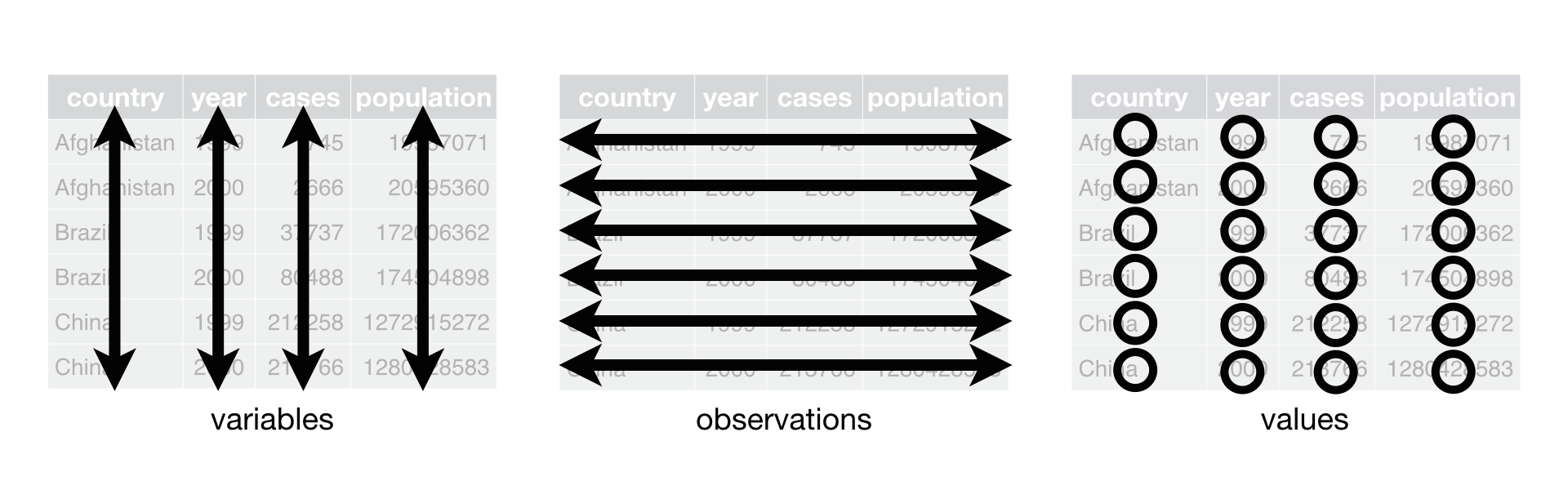
So going back to our dataset from before, we can see that it follows each of these three rules. Each person and each timepoint has their own rows (Rule 1). Every type of data measured (gender, age, etc.) has their own column (Rule 2), and each cell within the dataframe has only one value (Rule 3).
Let’s look at some examples where one or more of these rules are being violated.
data_untidy = [['tom', "26_m", 12, 15, 15],
              ['nick', "23_m", 10, 9, 12],
              ['julie', "18_f", 15, 13, 14],
              ['angela', "21_f", 10, 10, 12]]
df_untidy = pd.DataFrame(data_untidy, columns = ['name', 'age_gender', 'time1', 'time2', 'time3'])
df_untidy
| name | age_gender | time1 | time2 | time3 | |
|---|---|---|---|---|---|
| 0 | tom | 26_m | 12 | 15 | 15 |
| 1 | nick | 23_m | 10 | 9 | 12 |
| 2 | julie | 18_f | 15 | 13 | 14 |
| 3 | angela | 21_f | 10 | 10 | 12 |
In the example above, this dataset is messy because two variables (age and gender) have been coded into the same column. Having multiple variables in the same column in this way makes it much harder to calculate the average age of participants or get a gender breakdown for the sample.
But this can easily be fixed by splitting the column into two.
df_untidy[['age', 'gender']] = df_untidy.age_gender.str.split("_", expand=True)
del df_untidy['age_gender']

df_untidy
| name | time1 | time2 | time3 | age | gender | |
|---|---|---|---|---|---|---|
| 0 | tom | 12 | 15 | 15 | 26 | m |
| 1 | nick | 10 | 9 | 12 | 23 | m |
| 2 | julie | 15 | 13 | 14 | 18 | f |
| 3 | angela | 10 | 10 | 12 | 21 | f |
Here’s another case of untidy data, similar to one we’ve seen before.
data_messy = [['tom', 26, 12, 15, 15, 17, 18, 20],
              ['nick', 23, 10, 19, 12, 14, 11, 18],
              ['julie', 18, 15, 23, 14, 18, 12, 19],
              ['angela', 21, 10, 11, 12, 14, 15, 30]]
df_messy = pd.DataFrame(data_messy, columns = ['name', 'age', 't1_min', 't1_max', 't2_min', 't2_max', 't3_min', 't3_max'])
df_messy
| name | age | t1_min | t1_max | t2_min | t2_max | t3_min | t3_max | |
|---|---|---|---|---|---|---|---|---|
| 0 | tom | 26 | 12 | 15 | 15 | 17 | 18 | 20 |
| 1 | nick | 23 | 10 | 19 | 12 | 14 | 11 | 18 |
| 2 | julie | 18 | 15 | 23 | 14 | 18 | 12 | 19 |
| 3 | angela | 21 | 10 | 11 | 12 | 14 | 15 | 30 |
This dataset violates the rules of a tidy dataset because a) there’s more than one observation in each row, and b) we have multiple columns reflecting the same variable (the distinction between a minimum and maximum score).
But we can fix it using pd.melt with a combination of few other things. In this tidied version, we now see that each variable (name, age, time, min score, and max score) all have their own columns.
df_messy = pd.melt(df_messy, id_vars=['name', 'age'], var_name='time_minmax', value_name='score')

df_messy[['time','minmax']] = df_messy.time_minmax.str.split("_", expand = True)
del df_messy['time_minmax']

df_messy = df_messy.pivot_table(index=['name','age','time'], columns='minmax', values='score')
df_messy.reset_index(drop=False, inplace=True)
df_messy
| minmax | name | age | time | max | min |
|---|---|---|---|---|---|
| 0 | angela | 21 | t1 | 11 | 10 |
| 1 | angela | 21 | t2 | 14 | 12 |
| 2 | angela | 21 | t3 | 30 | 15 |
| 3 | julie | 18 | t1 | 23 | 15 |
| 4 | julie | 18 | t2 | 18 | 14 |
| 5 | julie | 18 | t3 | 19 | 12 |
| 6 | nick | 23 | t1 | 19 | 10 |
| 7 | nick | 23 | t2 | 14 | 12 |
| 8 | nick | 23 | t3 | 18 | 11 |
| 9 | tom | 26 | t1 | 15 | 12 |
| 10 | tom | 26 | t2 | 17 | 15 |
| 11 | tom | 26 | t3 | 20 | 18 |
Don’t worry if the actual code to make the data tidy doesn’t make sense right away (you will get there). We’ll talk more later about strategies you can use to wrangle data into tidy formats using Python. What you should be taking away from these examples is the differences in how these datasets are structured both before and after we tidied them.
Cleaning up and rearranging datasets is inevitable part of doing psychological research. Lots of data you work with may come to you in untidy formats, and you will have to clean that data up before you can analyze it. The good news is that knowing these principles of tidy, organized datasets will serve you well as you to start to design your experiments! The more you can build in tidy principles into how your data is recorded during the experiment, the more time you can save later when it comes to processing your data in Python.
Also importantly, this discussion highlights one major purpose of the Pandas library: namely to help you clean up and reorganize data. The commands like pd.melt() and pd.pivot_table() are pretty complex operations which alter your view of a dataset and make it easier to perform certain types of analysis. These reorganizations of data can be very difficult to do by hand but are facilitated by the dataframe library provided by Pandas.
6.11.2. A case example: organizing data for an psychological experiment#
The discussion so far might strike you as somewhat abstract. However, principles of data formatting and organization are very important for psychological research. Let’s consider the case most central to this course which is organizing a data file for a psychological experiment conducted on several participants composed of multiple trials and trial types. This is perhaps the most typical type of data format we will encounter in this work and is somewhat different from survey questions and other types of data which has a more complex structure often.
To keep things simple, let’s imagine that we are doing a decision making experiment. On each trial of the experiment the subject will be offered a choice between a gamble and a sure amount of money. For instance the subject might be presented with an option like “Would you prefer $10 now or a 50% chance to win 20 dollars otherwise nothing.” If you think about it a bit for this specific pair of options they on average give the same expected value because the expected value of the uncertain option is \(0.5*\$20 + 0.5*0 = \$10.\) If people were perfectly rational they should be indifferent between these two gambles. However, a common phenomena is that people show a biased called risk aversion where they prefer a certain reward over a risky gamble. Thus, even though on average you get the same, they do not want to take the gamble for the larger amount of money. There are several explanations of this but one intuitive one is that people don’t like regret and the feeling if you get nothing is so bad that makes people prefer the certain $10.
So imagine we do an experiment attempting to explore loss aversion. We might present people with several of these types of gambles across multiple trials. The reason is that we want more than one measurement and want to vary things like the probability of the higher reward on the risky gamble (e.g., instead of 50% chance we might want to explore 10% chance of winning). In addition, we might want to change the magnitudes of the rewards across different trials. Finally we will want to run multiple people so that our conclusions aren’t tied to one person. How should we structure our data file for this? You might think that we should first write the code for the experiment and then consider the data format. However, I find it is usually helpful to do the opposite. We start with the data format in mind right from the start.
Let’s look back at the key idea in a “tidy” dataset because we definitely want to be tidy here.
Each observation must have its own row (observations could be each person, each timepoint, etc.)
Each variable must have its own column (variables are some kind of measurement: gender, age, score, etc.)
Each value must have its own cell (value are the actual measurement: female, 23 years, 12 points, etc.)
So each observation would be a trial and so it needs its own row.
Each variable would be information about the trial, both the details of what the subject saw on that trial (e.g., the magnitude of the rewards and gambles) and also how they responded (reaction time, what choice they made, etc…).
Each value must have its own cell means that each of these numbers need to have their own column and not be combined. So let’s make a pretend dataframe from scratch to illustrate this example.
So let’s imagine that there are 10 stimuli in the experiment. We can denote them as the value of the certain option and then the value of the high and low reward for the gamble. This means each stimulus/trial in the experiment can be described with four numbers:
certain value
upper risky value
lower risky value
probability of upper risky value
We can fix a few alternatives (let’s say enough for 4 trials) using a python dictionary:
stim={"certain": [10, 15, 25, 50],
      "upper_risk": [20, 40, 30, 32],
      "lower_risk": [0, 23, 29, 0],
      "prob": [0.5, 0.5, 0.25, 0.75]}
Next we can pretend to generate some responses from one subject.
responses = {"reaction_time":[200, 400, 500, 600],
             "choice": [0, 1, 1, 0]}
Now we can build up a dataframe for one subject. We will do this by first defining a python dictionary called trials which includes all the variables associated with one measurement (trial number, the value of the certain gamble, the probabilty, etc…) as well as all the measurements made on that trial (response time, choice). These start out at the beginning of the cell as empy lists and then a for loop below fills them in.
subject_id = "some_subject_id0"

trials = {'subject_id':[],
          'trial_num':[],
          'certain':[],
          'upper_risk':[],
          'lower_risk':[],
          'prob':[],
          'reaction_time':[],
          'choice':[]}

for i in range(4):
    trials['subject_id'].append(subject_id)
    trials['trial_num'].append(i)
    trials['certain'].append(stim['certain'][i])
    trials['upper_risk'].append(stim['upper_risk'][i])
    trials['lower_risk'].append(stim['lower_risk'][i])
    trials['prob'].append(stim['prob'][i])
    trials['reaction_time'].append(responses["reaction_time"][i])
    trials['choice'].append(responses["choice"][i])

trials
{'certain': [10, 15, 25, 50],
 'choice': [0, 1, 1, 0],
 'lower_risk': [0, 23, 29, 0],
 'prob': [0.5, 0.5, 0.25, 0.75],
 'reaction_time': [200, 400, 500, 600],
 'subject_id': ['some_subject_id0',
  'some_subject_id0',
  'some_subject_id0',
  'some_subject_id0'],
 'trial_num': [0, 1, 2, 3],
 'upper_risk': [20, 40, 30, 32]}
The result is a python dictionary that includes column names and then the data that goes in the columns which is perfect for initializing a Pandas dataframe:
df=pd.DataFrame(trials)
df
| subject_id | trial_num | certain | upper_risk | lower_risk | prob | reaction_time | choice | |
|---|---|---|---|---|---|---|---|---|
| 0 | some_subject_id0 | 0 | 10 | 20 | 0 | 0.50 | 200 | 0 |
| 1 | some_subject_id0 | 1 | 15 | 40 | 23 | 0.50 | 400 | 1 |
| 2 | some_subject_id0 | 2 | 25 | 30 | 29 | 0.25 | 500 | 1 |
| 3 | some_subject_id0 | 3 | 50 | 32 | 0 | 0.75 | 600 | 0 |
This is great and shows a very natural way to structure the data from an experiment. Each trial is a row in the dataframe. Each column either describes what the stimulus was on that trial or the response from the participant. In addition two columns code the trial number and the subject idea. This is critical for analysis as we might be interested in order effects on trials and so we need to know which trials were first or last. In addition we want to keep subjects separate. Eventually we will build up a more complex dataframe that includes multiple subjects. For example:
stim={"certain": [10, 15, 25, 50],
      "upper_risk": [20, 40, 30, 32],
      "lower_risk": [0, 23, 29, 0],
      "prob": [0.5, 0.5, 0.25, 0.75]}

trials = {'subject_id':[],
          'trial_num':[],
          'certain':[],
          'upper_risk':[],
          'lower_risk':[],
          'prob':[],
          'reaction_time':[],
          'choice':[]}

def generate_subject_data(subject_id, trials):
    for i in range(4):
        trials['subject_id'].append(subject_id)
        trials['trial_num'].append(i)
        trials['certain'].append(stim['certain'][i])
        trials['upper_risk'].append(stim['upper_risk'][i])
        trials['lower_risk'].append(stim['lower_risk'][i])
        trials['prob'].append(stim['prob'][i])
        trials['reaction_time'].append(np.random.randint(200,1000))
        trials['choice'].append(np.random.randint(0,2))

for subj in ["some_subject_id0","some_subject_id1","some_subject_id2"]:
    generate_subject_data(subj,trials)

exp_df=pd.DataFrame(trials)
exp_df
| subject_id | trial_num | certain | upper_risk | lower_risk | prob | reaction_time | choice | |
|---|---|---|---|---|---|---|---|---|
| 0 | some_subject_id0 | 0 | 10 | 20 | 0 | 0.50 | 993 | 1 |
| 1 | some_subject_id0 | 1 | 15 | 40 | 23 | 0.50 | 587 | 0 |
| 2 | some_subject_id0 | 2 | 25 | 30 | 29 | 0.25 | 626 | 1 |
| 3 | some_subject_id0 | 3 | 50 | 32 | 0 | 0.75 | 835 | 0 |
| 4 | some_subject_id1 | 0 | 10 | 20 | 0 | 0.50 | 679 | 0 |
| 5 | some_subject_id1 | 1 | 15 | 40 | 23 | 0.50 | 205 | 1 |
| 6 | some_subject_id1 | 2 | 25 | 30 | 29 | 0.25 | 798 | 0 |
| 7 | some_subject_id1 | 3 | 50 | 32 | 0 | 0.75 | 742 | 1 |
| 8 | some_subject_id2 | 0 | 10 | 20 | 0 | 0.50 | 729 | 1 |
| 9 | some_subject_id2 | 1 | 15 | 40 | 23 | 0.50 | 790 | 0 |
| 10 | some_subject_id2 | 2 | 25 | 30 | 29 | 0.25 | 207 | 0 |
| 11 | some_subject_id2 | 3 | 50 | 32 | 0 | 0.75 | 526 | 1 |
Ok, take a careful look at this output. This is a dataframe with 3 subjects worth of data. The first column is the subject id. The second is the trial number but notice how it starts at 0 and counts up to 3 and then stops when a new subject id begins. Next is the stimulus definitions (certain, upper_risk, lower_risk, prob, etc…) and the responses. This is exactly the way people usually code a data file for a cognitive or perceptual experiment. It is “tidy” and includes all the information in a handy way we can use to analyze the data later. Here we generated the data with a simple program that I wrote in the cell above but generally we write a more complex program to handle this including showing the stimlus to the subject, recording their reaction time and so forth. This simple program is a proxy for that more complex program but shows you the important principle of how to organize your data in preparation for analysis. The analysis itself is what we will contemplate over the next several chapters.
6.12. The Split-Apply-Combine Workflow#
Perhaps one of the most common data analysis steps is known at the split-apply-combine workflow. Helping with this workflow is one of the more interesting and powerful features of Pandas (and other dataframe) libraries.
The split-apply-combine workflow refers to a very common sequence of data analysis steps that data analysts have to make. Usually a dataset arrives with multiple sub-units inside it. For example, we might get a .csv file that has all the trials of an experiment from several subjects. Often we want to perform analyses that aggregate across these various subject categories. For example we might want to analyze the performance of each subject. Or alternatively we might want to analyze the difficulty of each item on the test.
Both of these analyses require us to split the larger dataframe up into pieces and perform and analysis on each of these pieces. The step where you perform this analysis is called apply. So we break the bigger dataframe up into pieces, apply an analysis to each piece. The final step is to combine the results of those analyses back into a new dataframe structure for further analysis.
Fig. 6.1 tries to emphasize these steps:
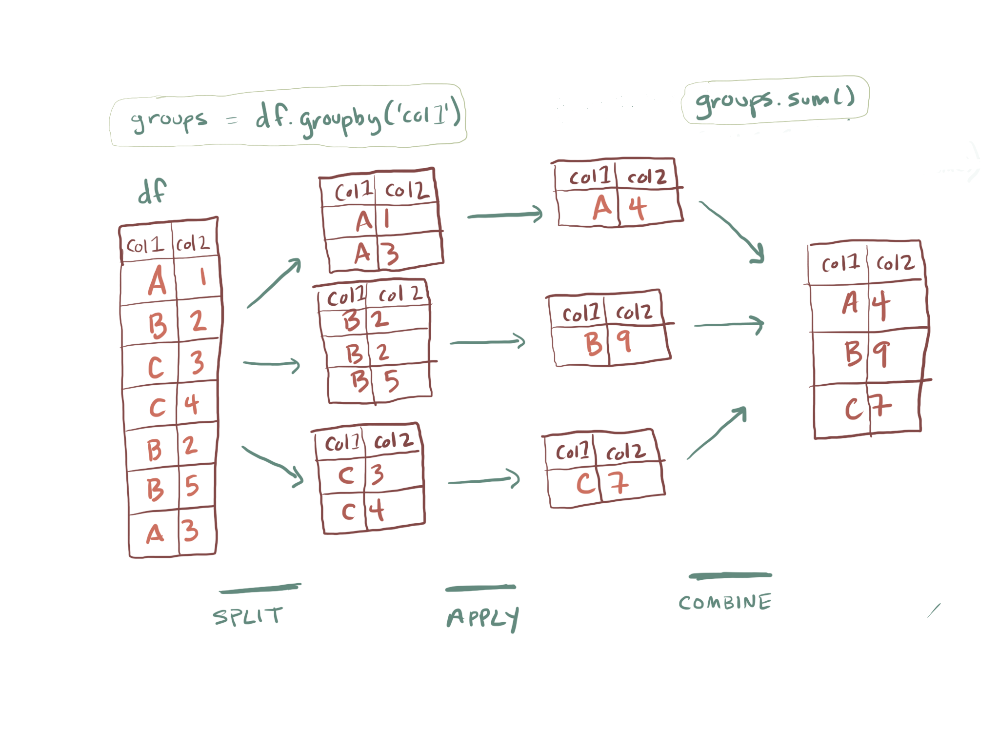
Fig. 6.1 Illustration of the split-apply-combine workflow!#
On the left we begin with our original dataframe (df) which has two columns. One column is categorical and takes on values ‘A’, ‘B’, or ‘C’ while the second column is numeric. The first step of the split-apply-combine workflow is that we might want to split the original dataframe into smaller groups based on the value of one or more of the columns. For this example it makes sense to break the original dataframe into smaller dataframes called “groups” based on the value of col1 (that is to say if the row is in category ‘A’,’B’, or ‘C’). The method that does this in Pandas is .groupby and we will discuss it in a moment. The result of the groupby operation is a partitioning of the original dataframe into smallers sets (called groups) which are the rows of the original dataframe just reorganized. The reorganization is such that all the rows that share the same value on the specified column are group together. For instance in Fig. 6.1 all the rows that had value ‘A’ in col1 are placed into the same group separate from all the rows that had value ‘B’ in col1 and so forth. This is the split operation.
Next there are several things we can do to each of the groups. We can iterate down them in a for loop for instance (more on that later) but also there are methods that will quickly compute various descriptives statistics to each group, or allow you to “apply” a custom function to each group. This custom function could be quite complex and so it allows you do do a lot of additional processing of the groups. The syntax for this tends to be very compact and helps to limit bugs so it is helpful to learn.
Let’s begin by the simple example in Fig. 6.1:
Here is the dataframe:
sac_df=pd.DataFrame({"col1":['A','B','C','C','B','B','A'],"col2": [1,2,3,4,2,5,3]})
sac_df
| col1 | col2 | |
|---|---|---|
| 0 | A | 1 |
| 1 | B | 2 |
| 2 | C | 3 |
| 3 | C | 4 |
| 4 | B | 2 |
| 5 | B | 5 |
| 6 | A | 3 |
Next we will group the rows by the values in col1:
sac_df.groupby('col1')
<pandas.core.groupby.generic.DataFrameGroupBy object at 0x11809eac8>
The result here doesn’t print out the individual groups but instead returns a pandas.core.groupby.generic.DataFrameGroupBy object. However we can print out the groups using iteration:
for name, group_df in sac_df.groupby('col1'):
    print(name)
    print('-----')
    print(group_df)
    print()
    print()
A
-----
  col1  col2
0    A     1
6    A     3


B
-----
  col1  col2
1    B     2
4    B     2
5    B     5


C
-----
  col1  col2
2    C     3
3    C     4
As you can see, the rows have been sorted into groups based on the value in col1. Since there are three distinct/unique values in col1 there are three groups here but if there were more distinct values there would be more groups.
Next we compute the sum() which applies the sum to each group. We can chain these operations in a sequence:
sac_df.groupby('col1').sum()
| col2 | |
|---|---|
| col1 | |
| A | 4 |
| B | 9 |
| C | 7 |
The result here is a new dataframe where the sum of the values of col2 for the different subgroups ‘A’,’B’, ‘C’ has been computed.
:::{tip} Check the results by hand to make sure you understand what has been calculated here! :::
Ok this example is fairly simple, what if we consider a more complex dataframe with more columns:
sac_df_2=pd.DataFrame({"col1":['A','B','C','C','B','B','A'],"col2":['A','A','A','B','B','B','B'],"col3": [1,2,3,4,2,5,3],"col4": [1.1,2.3,12.,16,22.21,9,0.5]})
sac_df_2
| col1 | col2 | col3 | col4 | |
|---|---|---|---|---|
| 0 | A | A | 1 | 1.10 |
| 1 | B | A | 2 | 2.30 |
| 2 | C | A | 3 | 12.00 |
| 3 | C | B | 4 | 16.00 |
| 4 | B | B | 2 | 22.21 |
| 5 | B | B | 5 | 9.00 |
| 6 | A | B | 3 | 0.50 |
If we .groupby() column 1 (col1) we get the same groups as before but notice they includes all the rows:
for name, group_df in sac_df_2.groupby('col1'):
    print(name)
    print('-----')
    print(group_df)
    print()
    print()
A
-----
  col1 col2  col3  col4
0    A    A     1   1.1
6    A    B     3   0.5


B
-----
  col1 col2  col3   col4
1    B    A     2   2.30
4    B    B     2  22.21
5    B    B     5   9.00


C
-----
  col1 col2  col3  col4
2    C    A     3  12.0
3    C    B     4  16.0
And now the apply-combine step computes the sum for all the numeric columns.
sac_df_2.groupby('col1').sum()
| col3 | col4 | |
|---|---|---|
| col1 | ||
| A | 4 | 1.60 |
| B | 9 | 33.51 |
| C | 7 | 28.00 |
Of course you don’t have to apply the sum to all the columns. If you just want to analyze col4 you can select it out before applying the sum:
sac_df_2.groupby('col1')['col4'].sum()
col1
A     1.60
B    33.51
C    28.00
Name: col4, dtype: float64
You can also group using more than one column as the grouping factors. For example in sac_df_2 there are actually two columns that have discrete values and so you might want to make groups that are all combinations of those two factors. If so you just pass a list of grouping columns to .groupby():
for name, group_df in sac_df_2.groupby(['col1','col2']):
    print(name)
    print('-----')
    print(group_df)
    print()
    print()
('A', 'A')
-----
  col1 col2  col3  col4
0    A    A     1   1.1


('A', 'B')
-----
  col1 col2  col3  col4
6    A    B     3   0.5


('B', 'A')
-----
  col1 col2  col3  col4
1    B    A     2   2.3


('B', 'B')
-----
  col1 col2  col3   col4
4    B    B     2  22.21
5    B    B     5   9.00


('C', 'A')
-----
  col1 col2  col3  col4
2    C    A     3  12.0


('C', 'B')
-----
  col1 col2  col3  col4
3    C    B     4  16.0
Then the sum operation will apply to all combinations.
sac_df_2.groupby(['col1','col2']).sum()
| col3 | col4 | ||
|---|---|---|---|
| col1 | col2 | ||
| A | A | 1 | 1.10 |
| B | 3 | 0.50 | |
| B | A | 2 | 2.30 |
| B | 7 | 31.21 | |
| C | A | 3 | 12.00 |
| B | 4 | 16.00 |
The output here looks a little different because the columns are organized hierarchically (the specific terms is that the index is hierarchical). But we can call .reset_index() a function we mentioned earlier to delete the hierarchical index and flatten things back to a standard data frame.
sac_df_2.groupby(['col1','col2']).sum().reset_index()
| col1 | col2 | col3 | col4 | |
|---|---|---|---|---|
| 0 | A | A | 1 | 1.10 |
| 1 | A | B | 3 | 0.50 |
| 2 | B | A | 2 | 2.30 |
| 3 | B | B | 7 | 31.21 |
| 4 | C | A | 3 | 12.00 |
| 5 | C | B | 4 | 16.00 |
The final result here is itself a dataframe and so can be use for further analysis and plotting.
6.12.1. Changing the “apply” step#
In the example we considered so far we summed the columns within in group. However there are actually several types of things you can do to groups in the “apply” step:
Aggregation: computes a descriptive statistic like a sum, mean, max, min, etc…
Transformation: perform a group-specific computation like standardsize (z-score) within a group
Filtration: discard data from small groups or filter data from a group based on the sum or mean in that group (e.g., removing outliers in a group)
6.12.1.1. Aggregation#
So far we computed the sum of columns within each group. However there are several other functions you can use. For example to compute the median instead:
sac_df_2.groupby('col1').median()
| col3 | col4 | |
|---|---|---|
| col1 | ||
| A | 2.0 | 0.8 |
| B | 2.0 | 9.0 |
| C | 3.5 | 14.0 |
Here is a list of common aggregation functions:
Function |
Description |
|---|---|
|
Compute mean of groups |
|
Compute sum of group values |
|
Compute group sizes |
|
Compute count of group |
|
Standard deviation of groups |
|
Compute variance of groups |
|
Standard error of the mean of groups |
|
Generates descriptive statistics |
|
Compute first of group values |
|
Compute last of group values |
|
Take nth value, or a subset if n is a list |
|
Compute min of group values |
|
Compute max of group values |
In addition there is a special .agg() (or .aggregate()) function that you can pass mulitple functions to from other libraries:
sac_df.groupby('col1').agg(np.sum)
| co32 | col4 | |
|---|---|---|
| col1 | ||
| A | 4 | 1.60 |
| B | 9 | 33.51 |
| C | 7 | 28.00 |
The previous example used the numpy np.sum() function. You can also provide multiple functions at once:
sac_df
| col1 | col2 | co32 | col4 | |
|---|---|---|---|---|
| 0 | A | A | 1 | 1.10 |
| 1 | B | A | 2 | 2.30 |
| 2 | C | A | 3 | 12.00 |
| 3 | C | B | 4 | 16.00 |
| 4 | B | B | 2 | 22.21 |
| 5 | B | B | 5 | 9.00 |
| 6 | A | B | 3 | 0.50 |
sac_df.groupby('col1').agg([np.sum, np.mean, np.std])
| col2 | |||
|---|---|---|---|
| sum | mean | std | |
| col1 | |||
| A | 4 | 2.0 | 1.414214 |
| B | 9 | 3.0 | 1.732051 |
| C | 7 | 3.5 | 0.707107 |
Which as you can see actually computes mutiple statistics on each group.
See also
You can read more about aggregation in the Pandos docs on Aggregation.
6.12.1.2. Transform#
Aggregation methods take in a grouped dataframe and compute a single number of statistics for each group. In contrast transform applies a function to a column and returns a column of the same size usually. This allows you to change the data within each sub group. A common version of this for behavioral science is to z-score data within a group to detect outliers, etc… Since that is the most common use case we’ll focus on that here.
sac_df_2.groupby('col1').transform(lambda x: (x-x.mean())/x.std())
| col3 | col4 | |
|---|---|---|
| 0 | -0.707107 | 0.707107 |
| 1 | -0.577350 | -0.875545 |
| 2 | -0.707107 | -0.707107 |
| 3 | 0.707107 | 0.707107 |
| 4 | -0.577350 | 1.089743 |
| 5 | 1.154701 | -0.214198 |
| 6 | 0.707107 | -0.707107 |
The transform function takes as argument a lambda function which is a way to write short one-line functions in python. This function takes 1 argument (x) which is the dataframe coresponding to each column of each group. It then computes the z-score of this data within the group and column and the result is combined into a new dataframe. This new data frame has the same column names as the original but we might want to rename them:
transformed_df=sac_df_2.groupby('col1').transform(lambda x: (x-x.mean())/x.std())
transformed_df=transformed_df.rename(columns={'col3':'col3_trans', 'col4': 'col4_trans'})
transformed_df
| col3_trans | col4_trans | |
|---|---|---|
| 0 | -0.707107 | 0.707107 |
| 1 | -0.577350 | -0.875545 |
| 2 | -0.707107 | -0.707107 |
| 3 | 0.707107 | 0.707107 |
| 4 | -0.577350 | 1.089743 |
| 5 | 1.154701 | -0.214198 |
| 6 | 0.707107 | -0.707107 |
To add these transformed columns back into our original data frame as new column we can use the .join() function which is like .concat() which we leared about earlier but combines the columns from a dataframe rather than appending the rows:
sac_df_2.join(transformed_df)
| col1 | col2 | col3 | col4 | col3_trans | col4_trans | |
|---|---|---|---|---|---|---|
| 0 | A | A | 1 | 1.10 | -0.707107 | 0.707107 |
| 1 | B | A | 2 | 2.30 | -0.577350 | -0.875545 |
| 2 | C | A | 3 | 12.00 | -0.707107 | -0.707107 |
| 3 | C | B | 4 | 16.00 | 0.707107 | 0.707107 |
| 4 | B | B | 2 | 22.21 | -0.577350 | 1.089743 |
| 5 | B | B | 5 | 9.00 | 1.154701 | -0.214198 |
| 6 | A | B | 3 | 0.50 | 0.707107 | -0.707107 |
The end result is that we z-scored col3 and col4 within the groups implies by col1.
See also
You can read more about aggregation in the Pandos docs on Transformation.
6.12.1.3. Filtration#
With the filtration apply step you provide a function that returns true or false for each group. Any group that the function returns True for is kept for the new dataframe and any group that returns False is dropped.
For example this step removes rows from the dataframe that belong to groups with only one or two members:
dff = pd.DataFrame({'A': np.arange(8), 'B': list('aabbbbcc')})
dff
| A | B | |
|---|---|---|
| 0 | 0 | a |
| 1 | 1 | a |
| 2 | 2 | b |
| 3 | 3 | b |
| 4 | 4 | b |
| 5 | 5 | b |
| 6 | 6 | c |
| 7 | 7 | c |
dff.groupby('B').filter(lambda x: len(x) > 2)
| A | B | |
|---|---|---|
| 2 | 2 | b |
| 3 | 3 | b |
| 4 | 4 | b |
| 5 | 5 | b |
Notice ‘a’ and ‘c’ entries have been removed because those groups have only two members each.
See also
You can read more about aggregation in the Pandos docs on Filtration.
6.13. Further Reading and Resources#
10 minute intro to pandas
A longer standalone video on how to use pandas
A visual guide to split-apply-combine strategies in Pandas by Towards data science
Split-Apply-combine strategy for data mining includes some additional facts and features of this approach
6.14. References#
- 1
Internally, pandas is primarily organized using columns. This just means that the computer code underneath pandas likes adding columns and hates adding new rows one at a time. It is just a thing. Thus, adding one row at a time is very inefficient. As a result it is usually best to get all your rows set and then create the dataframe.