Planning and Model-based Reinforcement Learning DRAFT

This chapter is a draft. It should not be considered complete or accurate.

Author

Todd M. Gureckis

Updated

October 7, 2026

Reading time

About 55 min

License

CC BY-NC-SAunless otherwise notedHow to cite

Print

PDF

Introduction

Some decisions are made by looking back. We choose the option that worked out well before, and the more often it paid off the more likely we are to pick it again. Other decisions are made by looking ahead. Before choosing a move in chess, a route across an unfamiliar city, or which job offer to accept, we think through what might happen if we took each option, what we could do next, and where that would leave us, and we reason forward to the choice that seems best. The work happens before the choice, and it does not necessarily require ever having made that choice before. This kind of forward thinking is what we will call planning.

Figure 1: Two ways to choose how to get to the airport. (a) Learning from the past. The traveler remembers how earlier trips by each option turned out and takes the one with the best record. (b) Planning ahead. The traveler runs each option forward in imagination: a taxi would get stuck in traffic and miss the flight, the bus stops everywhere and arrives late, and the subway takes one change and arrives on time. The person and the vehicles are from Twemoji, CC BY 4.0.

The learning methods we have focused on so far, TD learning and Monte Carlo methods, are a bit more like the first situation. They do not plan forward into the future. The value they assign to an action is a summary of what followed it in the past, and when the world changes they can only catch up by trying things again. However, there is a class of reinforcement learning algorithms that do plan. They estimate the value of an action by working out its likely consequences with a model of the environment, a representation of how the world works that is either given to the agent or learned from experience. This reading is about those algorithms and about whether, and how, people and animals use them.

We start with the computational view: how an agent can learn a model from its experience, how it can use the model to guide action in situations it has no direct experience with. We discuss why planning is hard, since the number of possible futures grows exponentially with how far ahead you look. Classic AI work, from the earliest search algorithms to the programs that beat the best players at chess and Go, focused on making this problem more tractable.

We then turn to how animals and people plan and use models. Do animals plan, or do they only repeat what has paid off before? How do people plan with far less computation than a full search would take, and how do they decide when thinking is worth it at all? What does planning look like in the brain?

Models and Planning

Many of the reinforcement learning methods we have met so far, such as TD learning and Monte Carlo methods, learn directly from experience and do not use a model of the world. Dynamic programming was the exception (solution methods). It assumed a model, the transition function $\mathcal{P}$ and reward function $\mathcal{R}$, which say how each action moves the agent from one state to the next and what reward each transition brings. A model is useful because it lets an agent know in advance what is likely to happen if it takes an action, without actually taking it. Using a model in this way, to work out the consequences of actions before acting on them, is planning. Model-based reinforcement learning asks how an agent can get such a model, and what it can do with one once it has it.

Model-free and model-based

A major distinction between reinforcement learning algorithms is whether they learn and use a model. Model-free algorithms, like the TD methods we have considered so far, do not. Model-based algorithms do. Having a model enables kinds of behavior that are difficult for model-free learning, in particular planning. Sutton & Barto, 2018 draw the relationship between learning and planning as a loop.

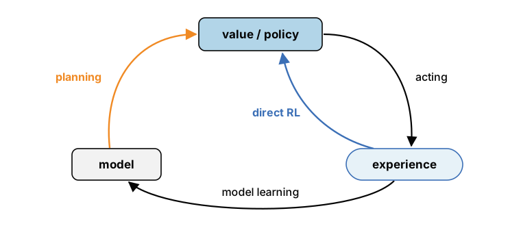
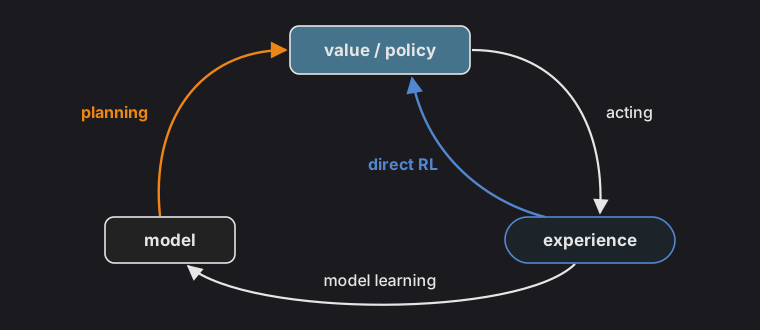
Figure 2: Experience, model, and value or policy. Acting produces experience. Direct RL (blue) updates the value function or policy from that experience. Model learning uses the same experience to improve a model of the environment, and planning (orange) uses the model to update the value function or policy without further experience. After Sutton & Barto, 2018, Chapter 8.

The loop has two routes from experience to the policy. On the direct route, experience updates the value function or policy, which is what TD learning and Q-learning do. On the indirect route, experience is used to learn a model, and planning then uses the model to work out what each action would lead to and so which action to take. A model-free agent has only the first route. A model-based agent can also consult its model when it decides, so a change in the world that it has learned about can change its choices before it has experienced the consequences of acting differently.

Dyna: learning and planning together

Perhaps the simplest way to put planning and learning together is Sutton's Dyna architecture (Sutton, 1991). A Dyna agent interacts with the world like a Q-learner, and every real step does three things. First, it makes an ordinary Q-learning update from the transition it just experienced. Second, it updates its model with the same transition, which in the simplest version just means remembering that taking action $a$ in state $s$ led to reward $r$ and state $s^{\prime }$. And, third, then it plans: it makes $n$ more Q-learning updates, each on a transition simulated from the model/memory, starting from a state and action it has experienced before and chosen at random.

Figure 3: The Dyna architecture. Real experience from interacting with the environment drives both a direct RL update (blue) and model learning. Search control picks states and actions from which the model generates simulated experience (dashed), and the planning update (orange) applies the same learning rule to simulated experience that the direct RL update applies to real experience. After Sutton & Barto, 2018, Chapter 8.

The tabular Dyna-Q algorithm

Initialize $Q(s,a)$ and $\mathit{Model}(s,a)$ for all $s\in \mathcal{S}$ and $a\in \mathcal{A}(s)$. Then loop forever:

1. $S\leftarrow$ the current (nonterminal) state.
2. $A\leftarrow \epsilon \text{-greedy}(S,Q)$.
3. Take action $A$, and observe the resulting reward $R$ and state $S^{\prime }$.
4. $Q(S,A)\leftarrow Q(S,A)+\alpha [R+\gamma \underset{a}{max}Q(S^{\prime },a)-Q(S,A)]$.
5. $\mathit{Model}(S,A)\leftarrow R,S^{\prime }$ (assuming a deterministic environment).
6. Repeat $n$ times:
   • $S\leftarrow$ a random previously observed state.
   • $A\leftarrow$ a random action previously taken in $S$.
   • $R,S^{\prime }\leftarrow \mathit{Model}(S,A)$.
   • $Q(S,A)\leftarrow Q(S,A)+\alpha [R+\gamma \underset{a}{max}Q(S^{\prime },a)-Q(S,A)]$.

Steps 1 through 4 are Q-learning. Step 5 learns the model, here by remembering the last outcome of each state-action pair, which is only correct if the environment is deterministic. Step 6 is planning: $n$ further Q-learning updates on transitions drawn from the model. After Sutton & Barto, 2018, Chapter 8.

If this looks familiar, it should. The experience replay that made DQN work stores past transitions in a buffer and trains the network on samples drawn from it, interleaved with new experience. Replaying a transition from a buffer and simulating it from a learned model are nearly the same operation, and in the tabular case they are identical, since Dyna's simplest model is a table of remembered transitions. The difference appears only when the model generalizes, so that it can produce transitions the agent has never experienced. The replay buffer, and the hippocampal replay it resembles, were explained as a way to interleave experience for a slow learner. Dyna uses the same operation to plan.

What does planning buy? A good place to see it is a small maze that Sutton and Barto use in their textbook (Sutton & Barto, 2018), six cells by nine with a few walls, in which the agent starts at S and receives a reward only on reaching G. The simulation below puts two agents in this maze side by side, one without planning ($n=0$), which is just Q-learning, and one with planning ($n=50$), and stops them halfway through their second episode.

planning steps

Without planning

episode 2, step 445last episode 2251 steps

With planning, 50 steps per move

episode 2, step 17last episode 893 steps

Figure 4: Greedy policies halfway through the second episode, in one run without planning ($n=0$) and one with planning ($n=50$). Arrows show the greedy action in each state whose action values are no longer all zero, and the yellow cell with the dot is the agent's current position. Without planning only the step into the goal has been learned. With planning the policy reaches almost back to the start. Simulation after Sutton & Barto, 2018, Example 8.1.

In the first episode both agents know nothing, so both wander until they stumble on the goal, typically several hundred steps for a path whose shortest version is 14. Planning cannot help yet, because the model holds no reward to pass back. Once each agent does reach the goal, however, the outcomes are quite different. The runs vary, but on the second episode the agent without planning typically wanders for hundreds of steps again, while the planning agent usually reaches the goal in a few dozen.

Without planning only one Q-value has changed (left), the one for the step that entered the goal. Every other step of the first episode ended in a state whose value was still zero, so it had nothing to pass back. With planning, that one piece of news is propagated backward through the model over and over while the agent takes each real step, and by the middle of the second episode the agent's policy reaches nearly back to the start. Most of the states it covers are ones the agent has not visited on this episode. The planning agent does with its model what the Q-learner can only do by walking the maze many times.

Press Run to let both agents carry on side by side, one real step at a time. A cell flashes when a planning update changes its arrow, so you can watch the news of the goal spread backward through the model while the planning agent walks. Reset starts both agents over with nothing learned, and the planning steps buttons set how many simulated updates the planning agent makes after each real step. After a reset the first episode can run for a long time before either agent finds the goal, so drag the speed slider to the right to hurry it along, or press Episode to finish the episode each agent is in at once.

The same advantage shows up in how fast each agent finds the shortest path. An agent with no planning steps needs about 25 episodes. With five planning steps per real step it needs about five, and with 50 planning steps about three.

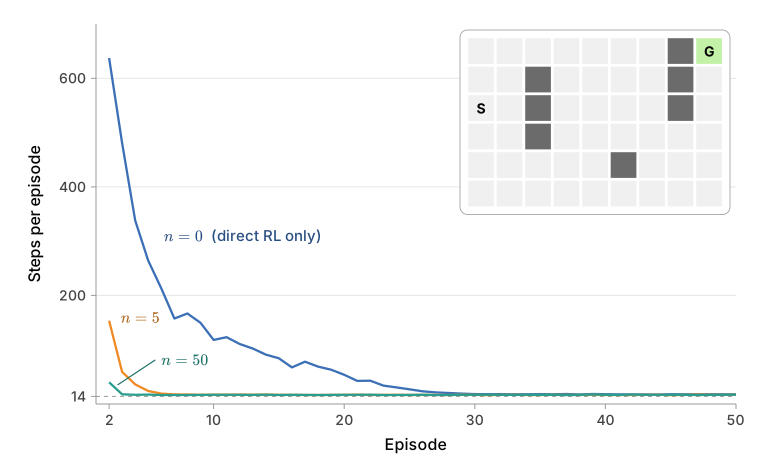
Figure 5: Learning curves in the Dyna maze (inset). The agent starts at S and is rewarded only at G. Each curve is the number of steps per episode for Dyna-Q with $n$ planning steps per real step, averaged over 100 runs. The curves settle a few steps above the shortest path of 14 because the agent keeps exploring. The first episode is omitted, since its length does not depend on $n$. Simulation after Sutton & Barto, 2018, Example 8.1.

A key lesson of Dyna is that an agent can learn something useful before it has encountered any reward. During the first episode the planning agent's values stay at zero, but its model is filling in with how the maze is laid out, and that knowledge is what lets a single reward spread so quickly once it arrives. Learning about the structure of the world without reward is an issue we will return to, surprisingly, when we talk about rats.

Planning at decision time

Dyna plans in the background. Its simulated updates improve a cached value function for every state the model can reach, whether or not the agent is anywhere near them. The alternative is to plan now, for the state you are in: simulate forward from the current state with the model, look at where each possible action leads and where the actions after those lead, and choose the action whose simulated futures look best. This is decision-time planning, and it is what a chess player does when thinking about the next move. It spends computation only on the part of the problem that is relevant at the moment, and it can use a model that has just changed, because nothing is cached. What it explores is a tree like this one:

Figure 6: A search tree unrolled from the current state $s_t$. Open circles are states, filled circles are actions, and T marks a terminal state. Each level of the tree multiplies the number of paths by the number of available actions. After Sutton & Barto, 2018, Chapter 8.

The problem is the size of the tree. With $b$ actions available in each state, looking $d$ steps ahead means considering $b^d$ sequences. In Go the first player has 361 legal moves, the second has 360 replies to each of them, and so on, so that even a few moves ahead the tree has more branches than any computer could visit. Some way of deciding which parts of the tree deserve attention is not an optional refinement. Without one, decision-time planning is impossible in any interesting problem.

Classical search

AI has faced this problem since its beginning. Newell and Simon described problem solving as search through a space of states, from a starting state to a goal, using operators that turn one state into another (Newell & Simon, 1972). Classical planning grew out of that work into a large subfield with its own history (Ghallab, Nau & Traverso, 2016), and the basic search algorithms are the first thing taught in most introductions to AI (Russell & Norvig, 2010). They assume what most decision-time planning assumes, a known model that can say which states follow from which, and they differ in only one respect: which node of the tree to look at next.

Classical search does not solve quite the problem a reinforcement learning agent faces. It looks for a path to a goal, a state that passes a test, and it can stop as soon as it finds one. A reinforcement learning agent has no single goal. Rewards can arrive anywhere along a path, different endings are worth different amounts, and what the agent wants is the action with the highest expected return, not any path that ends well. It cannot stop at the first good leaf, since a better one may lie elsewhere in the tree, and it has to compare the leaves it finds by backing their values up toward the root. However, the question classical search answers, which part of the tree to look at next when you cannot look at all of it, is the same one, and its answers carry over. We go through them for that reason, as a set of ideas about how a tree can be explored.

The simplest answer is to look at every node at one depth before moving to the next. This is breadth-first search(?), and it is guaranteed to find the goal that is the fewest steps away. However, it has to keep the whole frontier of the search in memory, and with $b$ actions per state the frontier at depth $d$ holds $b^d$ nodes. Depth-first search makes the opposite choice. It follows one branch all the way down, and only when that branch ends does it back up to the most recent choice and try the next action there. It needs to remember only the path it is on, which is very little memory, but it can spend a long time far down a bad branch, and in a tree with no bottom it may never come back. Iterative deepening combines the two by running depth-first search with a depth limit of one, then two, then three, and so on (Korf, 1985). It repeats the shallow parts of the tree on every pass, but because most of the nodes in a tree are in its deepest level, the repetition costs little, and it gets the small memory of depth-first search and the shortest-path guarantee of breadth-first search.

step 13

The frontier is a queue: new nodes join the back.

The frontier is a stack: new nodes go on top.

The frontier is sorted by g + h, smallest first.

Figure 7: The order in which three searches visit the same tree, stopping at the goal (teal). (a) Breadth-first search finishes each level before starting the next. (b) Depth-first search follows the leftmost branch to the bottom and backs up. Both look only at the structure of the tree and so visit most of it. (c) A* expands the node with the smallest $g+h$, where $g$ is the number of steps taken and $h$ an estimate of the number left. Dashed nodes were generated but never expanded.

Press Run or Step to watch the three searches side by side. Each keeps a frontier of nodes it has generated but not yet visited (dashed, numbered by their place in line), and on every step it visits the first node in line (highlighted). The three searches differ only in how they order the line.

Breadth-first and depth-first search are blind. They use the model to find a state's successors, but never to judge whether a successor looks closer to the goal, so they visit most of the tree before they stumble on it. Best-first search keeps its frontier sorted by an estimate of how promising each node is and always expands the best one. The best known version is A*, which scores a node $n$ by

$$\begin{array}{}\text{(1)}& f(n)=g(n)+h(n)\end{array}$$

where $g(n)$ is the cost of the path from the start to $n$ and $h(n)$ is a heuristic(?) estimate of the cost from $n$ to the goal (Hart, Nilsson & Raphael, 1968). If $h$ never overestimates the true cost, the first goal A* reaches is guaranteed to be the best one, and the closer $h$ is to the truth, the fewer nodes it needs to expand. A heuristic is a value function under another name. It is an estimate, computed ahead of time, of how good it is to be in a state. With a perfect heuristic A* walks straight to the goal and the search is unnecessary, and with $h=0$ it falls back to a blind search that grows outward by cost. Heuristic search is therefore the oldest version of an idea that comes up again and again in this chapter, a cached estimate of value deciding where an expensive search should look.

Monte Carlo tree search

One way to avoid searching the full tree is to sample it. From the current state, use the model to simulate many episodes to the end, choosing actions at random, and average the returns for each first action. This is a Monte Carlo method in the same sense as the Monte Carlo methods for estimating value: the value of an action is the average return of episodes that begin with it. However, it wastes most of its effort. In a typical state there may be many possible actions but only one or two good ones, and random playouts spend nearly all their time on the others.

Monte Carlo tree search (MCTS) fixes this by treating the choice at every state in the tree as a multi-armed bandit (Kocsis & Szepesvári, 2006; Coulom, 2006). Simulation effort then flows toward the actions that look promising, just as a good bandit strategy spends its pulls on the arms that look good, while still trying the others from time to time in case their early results were unlucky. To do this it keeps a tree of statistics, one node for each state it has visited, and each node records how many simulations have passed through it and the total return of those simulations. Their ratio is the node's average return.

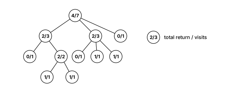
Figure 8: The tree of statistics that MCTS keeps. Each node is a state reached by a sequence of actions from the root, and it records the total return of the simulations that passed through it over the number of them. Here every simulated episode ends with a return of 1 or 0, so 4/7 at the root means that four of seven simulations succeeded. With other rewards a node adds up returns the same way, and the ratio is its average return $Q$.

Each iteration grows the tree by one node and simulates one episode, in four steps:

Figure 9: One iteration of Monte Carlo tree search. (a) The tree policy selects a path down the existing tree (highlighted), choosing the child with the highest UCT score at each level, and (b) expands it by one node. (c) The default policy simulates an episode from the new node to the end, here one with a return of 1, and none of the states it passes through are added to the tree. (d) The return is backed up along the selected path, adding 1 to the total and one visit to every node on it. After Browne et al., 2012.

Selection is where the bandit comes in. At each node the search descends to the child that maximizes

$$\begin{array}{}\text{(2)}& Q(\text{child})+c\sqrt{\frac{\ln N(\text{parent})}{N(\text{child})}}\end{array}$$

where $Q(\text{child})$ is the average return of simulations through that child, $N$ counts visits, and $c$ sets how much weight exploration gets. This is the UCB rule for bandits, with each child playing the part of an arm, so children that have been tried rarely relative to their siblings get a bonus that shrinks as they are visited. In a tree it is called UCT (Kocsis & Szepesvári, 2006). The new node is then valued by a cheap random playout, and its return is added to every node on the path, as the figure shows.

1. Selection2. Expansion3. Simulation4. Backpropagation

The tree starts as just the root, R. Each node will show its total return over its number of visits. Press Step to begin.

iterations 0

Figure 10: Monte Carlo tree search, step by step. The search starts with a tree that is only the root and adds one node per iteration, running UCT on a small game in which every move has a hidden value and an episode succeeds if the values along it add up to enough. Once the tree is too wide to label, edges thicken with the number of simulations that passed through them. In print, the panel shows the tree after 150 iterations, by which point the search has found lines under A that succeed and spends most of its simulations on them.

Press Step to run the search one step at a time. Selection goes down one level per step, tagging each child it compares with its UCT score, and backpropagation updates one node per step on the way back up. The line under the tree says what each step did. Iteration finishes the iteration on screen, and +50 runs fifty at once. The first iterations fill in the root's three children, and for a while the search spreads its simulations across all of them. As playouts under A succeed more often, selection returns there more and more, and the counts along its best lines pull away from the rest.

Two-player games

MCTS made its name in games such as Go, where two players take turns and a result that is good for one is bad for the other. The algorithm is the same, except for the backup. Each node keeps its statistics from the point of view of the player whose move led to it, so a playout that the first player wins is added as a win at the nodes where that player moved and as a loss at the nodes where the opponent moved. Selection then picks, at every level, the move that is best for the player whose turn it is.

As iterations accumulate, the tree grows asymmetrically. Promising lines of play are visited often and explored deeply, and poor ones only as often as the exploration bonus requires. When the time for thinking runs out, the algorithm takes the action at the root that has been visited most. MCTS needs no heuristic evaluation function, only a model that can simulate forward, and it can be stopped at any time with a sensible answer, two properties that made it the dominant method for game playing in the decade before deep learning.

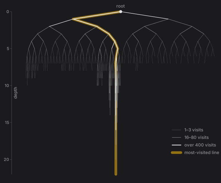
Figure 11: A tree grown by MCTS after 5,000 iterations of UCT on a simple synthetic problem, a binary tree in which every action adds a hidden amount to the episode's score and an episode succeeds if the total is high enough. The first few levels are searched evenly. Below them, simulation effort concentrates on a few promising lines, which are explored far more deeply than the rest. The yellow line is the one the search visited most. After Browne et al., 2012.

AlphaGo, which beat the world champion Lee Sedol in 2016, combined MCTS with deep networks of the kind behind DQN (Silver et al., 2016). A policy network, trained first on human games and then by self-play, proposed moves, so that selection concentrated on moves a strong player would consider. A value network, trained to predict the winner from a position, evaluated new nodes, and its estimate was mixed with the outcome of fast rollouts. AlphaGo Zero dropped the human games and the rollouts altogether, using a single network trained only by self-play to guide the search and evaluate positions (Silver et al., 2017). The result is a clean division of labor between the two kinds of reinforcement learning. Cached, model-free knowledge in the networks tells the search where to look and when to stop. Model-based search then does what the cache cannot, which is to check its suggestions against the actual consequences of the moves.

Model-Based and Model-Free Control in Animals

The ideas about planning and model-based learning covered above primarily derive from research in computer science and artificial intelligence. However, they have had important impact on thinking about human and animal behavior. A basic question is if animals and human learn models of the world, and how could we tell?

The habit machine

Thorndike's law of effect says that a response followed by satisfaction becomes more firmly connected to the situation in which it was made, so a cat that escapes a puzzle box is a little quicker next time to repeat whatever opened the door (Thorndike, 1911).

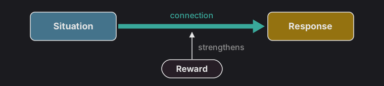
Figure 12: The stimulus-response account of the law of effect. Reward strengthens the situation-response connection, drawn here as the width of the arrow, but is not itself stored. After Thorndike, 1911.

On this account a cat does not press a lever for the food. It presses because pressing, in that situation, has been stamped in. A Q-learner is in the same position. It knows that $Q(\text{box},\text{press})$ is high, and that is all. You can think of it as a habit — something you do automatically without thinking partly because it has been successful before.

Not every psychologist accepted that this is all an animal learns.

The main alternative view (described by Tolman, Rescorla, Colwill, and Dickinson among others) argued that animals learn more general expectancies about the consequences of their actions. On this account the rat learns that pressing the lever produces food, an association between the response and its outcome, and the box tells it when that relation holds. The structure is usually written S-R-O, for situation, response, and outcome (Colwill & Rescorla, 1986). The difference from the stimulus-response account is what happens to the reward. Here it does not do its job and disappear. A representation of the particular outcome, this food and not just something good, becomes part of what is learned, and whether the rat presses depends on how much it wants that food at the moment it chooses.

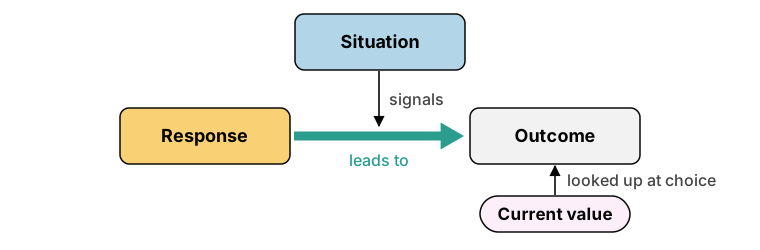
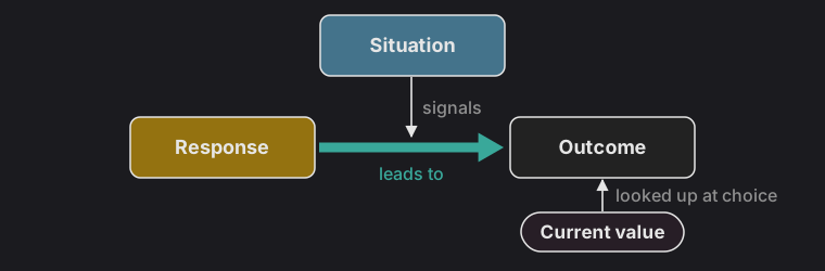
Figure 13: The stimulus-response-outcome account. The response is connected to its outcome, the situation signals that the response will produce that outcome, and the value of the outcome is looked up when the animal chooses. After Colwill & Rescorla, 1986.

If animals were simply S-R learning, habit machines, what would follow? They would learn nothing about an environment in which they receive no reward, because without reward there is nothing to stamp in. And they could not respond to a change in the value of an outcome until they had experienced the consequence of acting under the new conditions, because the estimated value of the action knows nothing about what the action leads to. Both predictions have been tested, and both turn out to be wrong, at least some of the time.

Tolman, latent learning, and cognitive maps

Tolman spent most of his career at Berkeley arguing against the stimulus-response psychology of his day. Along the way he explained several puzzling findings with rats in mazes, from his own lab and from others. One interesting study was by Blodgett, who ran three groups of hungry rats through a six-unit maze, once a day (Blodgett, 1929). The first group found food in the goal box from the first day. The other two found nothing there for the first few days, and were simply taken out of the maze when they reached it. For one of these groups food was introduced on the third day, and for the other on the seventh.

Figure 14: Latent learning. (a) Blodgett's six-unit alley maze, seen from above. One-way doors (D) kept the rats from retracing their steps, and an error was an entry into a blind alley. (b) Errors per day for three groups. Group I found food in the goal box from the first day. Groups II and III found nothing until day 7 and day 3 respectively. Open circles mark days without food and filled circles days with it. The day after the unrewarded groups first found food their errors dropped almost to the level of the group that had been rewarded all along. Tolman and Honzik found the same with a longer maze (Tolman & Honzik, 1930). Redrawn from data in Blodgett, 1929, as reprinted in Tolman, 1948.

The unrewarded rats improved a little while they wandered, as rats do. The interesting thing is what happened on the day after they first found food. Their errors dropped abruptly, almost to the level of the group that had been rewarded all along. A habit machine cannot do this. It would have to learn the route one prediction error at a time, starting from the goal and working back toward the start, and that takes as many days as it took the first group. The rats evidently did not need to. They had been learning the maze all along, and the reward only gave them a reason to show it. Tolman called this latent learning(?).

Tolman's interpretation was that the rats had formed a cognitive map(?) of the maze, a representation of its routes and the relations between places, and that behavior was then directed by the map toward whatever the animal wanted (Tolman, 1948). In the stimulus-response psychology of the time this was a heretical idea, partly because it was not clear what a map in a rat's head could be, or how it could be used. Framed computationally, the rats had learned something about the transition function of the maze, which choice point leads to which, without any reward to drive the learning. When reward appeared at the end, an agent with that knowledge could compute a good route at once, without having to learn one. This is what the Dyna agent did in its maze. Until it first reached the goal every value stayed at zero, but its model was filling in with the layout, and when the first reward arrived planning spread it back toward the start within a single episode. In both cases much of the learning happens before there is any reward to learn about.

Outcome devaluation

Latent learning shows that animals learn more than values. A second line of work, begun by Adams and Dickinson, shows that they use what they know about outcomes when they choose (Adams & Dickinson, 1981). The clever design has three phases. First, rats learn to press a lever for a particular food. Then the food is "devalued," meaning that something the rats previously found rewarding is made undesirable. This happens away from the lever, either by pairing it with illness (an injection of lithium chloride after the rats eat it) or by letting the rats eat it until they are sated. Finally the lever is returned, but pressing it no longer delivers any food (a test "in extinction"), so the rats cannot learn anything new about the consequences of pressing during the test itself. Consider what each kind of agent predicts. A habit machine has a cached value for pressing the lever, and nothing that happened in the second phase touched it, so it should press at the same rate as control rats whose food was left alone. An agent that represents what pressing leads to, and what that outcome is now worth, can put the two together and conclude that pressing is no longer a good idea, without ever having pressed the lever for poisoned food.

After moderate training the rats behave like the second kind of agent, and press much less than controls. However, the result depends on how much the rats were trained. After extensive training, the rats keep pressing a lever for a food they no longer want, and will not eat if it is given to them (Adams, 1982). The same animal, performing the same response, appears to be controlled by knowledge of the outcome early in training and by something that ignores the outcome later.

Figure 15: Outcome devaluation. (a) The design: training, devaluation of the food by illness or satiety (with an undevalued control), and a test in which pressing delivers no food. (b) Lever presses per minute in the test. After moderate training (2 sessions), rats whose food was devalued press much less than rats whose food was not. After extensive training (10 sessions) they press as much or more, even though the food is no longer wanted. After Niv, Joel & Dayan, 2006, a schematic of results like those of Adams, 1982. The rat, cheese, and syringe are from Twemoji, CC BY 4.0.

Behavior that is sensitive to the current value of its outcome is called goal-directed(?) and it more like S-R-O learning. Behavior that is insensitive to it is called a habit(?), and extended practice shifts behavior from the first to the second. So animals seem to exhibit behavior both consistent with the "habit machine" and also quite different and more flexbiel. In the language of reinforcement learning, that later type of learning may be like using a model which knows the probability of next states following an action and rewards.

Two systems: model-based and model-free control

The rats in the devaluation experiments were goal-directed early in training and habitual after extensive training. Daw, Niv & Dayan, 2005 gave the distinction a computational reading. The goal-directed system is a model-based planner. It represents the task as a tree of states and actions and evaluates an action by searching forward through the tree to the outcomes it leads to. The habitual system is a model-free learner that caches a value for each action. If the food is devalued, the tree system finds the change as soon as it next searches, because the value of the food is part of the tree. The cache has stored $Q(S_0,\text{press})=1$, has no way to connect that number to the food, and keeps recommending pressing until pressing has been followed, often enough, by an outcome that is no longer rewarding.

Figure 16: Two systems for the same lever-pressing task. (a) The tree system represents the states, the actions available in each, and where they lead, and evaluates an action by searching forward to the outcomes. (b) The cache system stores a value $Q$ for each action in each state, learned from experience, and never represents where the actions lead. After Daw, Niv & Dayan, 2005.

Why have two different learning systems? Daw and colleagues' answer is that each system is best in different circumstances. Forward search makes efficient use of experience, since a single new fact about an outcome changes the value of every action that leads to it, but it is computationally costly and it is noisy when the tree is deep, because small errors accumulate over many steps of search. Caching is cheap (you don't have to think through the tree), but it learns slowly, because values have to be passed back from the outcome one prediction error at a time. So forward search should do well early in training by learning quickly but remains error prone the cached Q-values should asymptote well after extensive training.

That leaves the question of how to choose when the two disagree. Their answer is that the brain should trust whichever system is more certain of its recommendation. The two systems are uncertain for different reasons. The tree system's uncertainty comes from the computational noise of searching. The cache's comes from how little experience it has had, and it falls with training. Early on, the cache knows little and the tree system wins. After extensive training the cache is accurate and the tree system's noise makes it the less reliable of the two, so control passes to the habit.

The two-step task and the cost of planning

The devaluation test is hard to run with people, since an experimenter cannot poison a participant's food for force feed them. To study the interaction between these learning processes in humans, Daw and colleagues designed a task that separates model-based from model-free control in a simple bandit-like task (Daw et al., 2011). On each trial the participant makes two choices (Figure 17a). At the first stage they choose between two options. Each leads to one of two second-stage states, but not deterministically: one option leads to the blue state 70% of the time (a common transition) and to the pink state 30% of the time (a rare transition), and the other the reverse. At the second stage they choose again between two options, and each of these pays a reward with a probability that drifts slowly over the course of the experiment, so that participants have to keep learning.

Figure 17: The two-step task. (a) Common (solid, 70%) and rare (dashed, 30%) transitions from each first-stage choice; second-stage payoffs drift (inset). (b) People's stay probabilities, from Daw et al., 2011, with standard errors. Staying is more likely after a reward, and the effect of reward depends on the transition. (c) A simulated model-free learner repeats a first-stage choice that was followed by reward, whatever the transition. (d) A simulated model-based learner's tendency to repeat depends on the interaction of reward and transition type, and after a reward that followed a rare transition it usually switches. Both learners have a learning rate of 0.5 and an inverse temperature of 5, and the dashed line marks chance. After Daw et al., 2011 and Otto et al., 2013.

The analysis looks at whether a participant repeats their first-stage choice on the next trial. Suppose the last trial's first-stage choice led, by a rare transition, to the pink state, and the participant was rewarded there. A model-free learner credits the first-stage choice with the reward and is more likely to repeat it, as it would after any reward (Figure 17c). A model-based learner reasons differently. The pink state is good right now, and the most reliable way to get there is the other first-stage option, which leads to pink 70% of the time. So after a reward that followed a rare transition it should switch, and after a lack of reward that followed a rare transition it should stay (Figure 17d). A model-free learner's stay probabilities show only a main effect of reward. A model-based learner's show an interaction between reward and transition type. People show both, a main effect and an interaction (Figure 17b), which is usually modeled by mixing the two learners' values before a softmax,

$$\begin{array}{}\text{(3)}& Q_{\text{net}}(a)=w{Q}_{\text{MB}}(a)+(1-w)Q_{\text{MF}}(a)\end{array}$$

where $w$, the model-based weight, measures how model-based a person is. There was also a neural surprise. Prediction errors in the striatum, long associated with model-free TD errors, reflected model-based as well as model-free values. So the two systems are not cleanly separate in the brain. Model-based values reach the same learning signal the cache uses, one hint that the model may train the cache.

If model-based control is costly, it should suffer when a person's cognitive resources are taken up with something else. Otto and colleagues tested this by having people perform the two-step task while also doing a demanding secondary task that loaded working memory, on some trials and not others (Otto et al., 2013). On trials with no load for the last two trials, people's choices showed the interaction that marks model-based control (Figure 18a). On trials with a load on the current trial or the one before, the interaction disappeared, and only the main effect of reward remained. Load, in effect, lowered $w$.

Figure 18: Working memory load and model-based choice. Trials are sorted by when the most recent secondary task occurred: two trials back (a), on the previous trial (b), or on the current trial (c). Error bars are standard errors. Redrawn from data in Otto et al., 2013, Experiment 1.

So planning is not only noisy when the tree is deep, as the arbitration account emphasizes. It also draws on limited executive resources that are needed for other things. A cheap system that takes over when those resources are busy earns its keep even if it is sometimes wrong. The same idea has a clinical version. If habits are what behavior falls back on when goal-directed control fails or is overwhelmed, then disorders marked by compulsive, outcome-insensitive behavior, such as addiction and obsessive-compulsive disorder, might be understood in part as an imbalance between the two systems, and the two-step task has been used widely to look for a reduced $w$.

How People Plan

The previous discussion highlights that humans and other animals might be sensitive to the outcomes of their choices, in addition to their incrementally learned value. However, the planning algorithms we considered earlier were about exploring large trees of future possibilities. An interesting line of research has explore the cognitive algorithms that people use for multi-step planning in richer and more complex tasks. Much of this builds on research of how people play games because game have a clear tree of possible game states.

Lessons from chess

Chess has been studied more than any other game in cognitive science. Simon and Chase called it the psychologist's "Drosophila," a standard task around which knowledge could accumulate (Simon & Chase, 1973), and it is a good place to look for planning because the tree is far too large for anyone to search. The first surprise came from de Groot, a Dutch psychologist and a strong player himself, who asked players from grandmasters to club players to think aloud while choosing a move (de Groot, 1965). The grandmasters did not search noticeably more positions or look noticeably further ahead than the weaker players. They also often came back to the same few lines again and again, each time a little deeper. What distinguished them was which moves they considered in the first place: the good moves were among their first thoughts, and they spent their search checking them.

De Groot traced this to perception. Shown a position from a real game for a few seconds, a master could put back almost all of the pieces, and a weaker player far fewer, a finding Chase and Simon later showed largely disappears when the pieces are placed at random (Chase & Simon, 1973). The master's advantage was not a better memory or a deeper search but knowledge of familiar configurations of pieces, many of which come with a good move attached. In the language of this chapter, that knowledge is a learned cache that tells the search where to look. Computational cognitive scientists have taken this further, building models of the specific algorithms that support planning and asking how they change with learning and expertise.

Human tree search

Van Opheusden and colleagues studied this question in a game chosen to be hard enough to require planning and simple enough to model (van Opheusden et al., 2023). In four-in-a-row, a relative of tic-tac-toe played on a board of four rows and nine columns, players take turns placing pieces, and the first to get four in a line wins. Pieces can go on any empty square. You can play it below against a computer that does no planning at all. It looks only at its own next move: it takes a win if there is one, blocks a square where you would win, and otherwise plays whatever move a simple heuristic scores best. Because it never looks past its own move, you can beat it by setting up two threats at once, since it can block only one.

first move

you 0 · computer 0 · draws 0

Your move.

You play black. Click any empty square; pieces do not drop to the bottom.

Figure 19: Four-in-a-row on a 4 by 9 board, against an opponent that looks one move ahead and no further. It scores boards with the same kind of heuristic as the model in Figure 20, but never searches. After van Opheusden et al., 2023.

The model of a player has two parts, and they correspond to the two parts of A*. The first is a heuristic, a function that scores a board without looking ahead at all (Figure 20a). It counts simple patterns for each player, such as two pieces next to each other, two with a gap between them, and three in a row with the fourth square still open, counting a pattern only where four in a row could still be completed. Each count is multiplied by a weight, and pieces near the center add a little more. From black's point of view,

$$\begin{array}{}\text{(4)}& V(s)=w_{\text{center}}{V}_{\text{center}}(s)+c_{\text{black}}\sum _i{w}_i{f}_i(s,\text{black})-c_{\text{white}}\sum _i{w}_i{f}_i(s,\text{white})+ϵ\end{array}$$

where each feature $f_i$ is 1 if a pattern appears at a particular place and orientation, and $ϵ$ is noise. The weights $w_i$ depend only on a pattern's type and are fitted to each person. The constants $c$ make the patterns of the player whose move it is count for more, since three in a row is an immediate win on your own move but can be blocked on your opponent's. Like $h(n)$ in A*, $V(s)$ is a cached estimate of how good a position is.

The second part is a search that uses the heuristic to decide where to look (Figure 20b). Starting from the current board, the model repeats three steps. It follows the most promising line of play down the tree it has built so far, choosing at each level the move that currently looks best for the player whose turn it is. It expands the position at the end of that line, generating the moves available there and scoring each new position with the heuristic. And it backs the new scores up the tree, on the assumption that each player picks the move that is best for them, so that a position is worth as much as the best move available from it. In the example, black's best-looking move makes three in a row and scores 3.7. Expanding it shows that white can block, and white's best reply leaves black with only 0.3. That value is backed up, and black's other candidate, worth 2.5, becomes the best move at the root, which is where the next pass will look. Each pass extends the tree wherever it currently looks best, so the search runs deep along a few promising lines and leaves most of the tree unexplored. After each pass the search stops with some probability, which makes the amount of planning a fitted parameter too, and the model then plays the move at the root with the highest value.

Figure 20: How the four-in-a-row model chooses a move. (a) The heuristic counts patterns for each player (lines on the board), weights them, and adds a term for pieces near the center; the weights here are examples. (b) Two passes of best-first search from the same board, with each new piece highlighted. The first pass scores black's best moves. The second expands the best of them, which makes three in a row, into white's best replies. White's best reply blocks it, its value is backed up, and black's other move becomes the best one at the root (bold arrow). After van Opheusden et al., 2023, Figure 1.

To make it a model of a person and not an engine, moves that the heuristic scores far below the best are pruned without being explored, some features are randomly overlooked on each move, values are perturbed by noise, and once in a while the model lapses and plays a random move. Because the search is noisy, the probability of each move a person made was estimated by running it many times. Fitted to people's moves this way, it predicts which move a person will make far better than simpler alternatives, and removing any of its components makes it worse.

Figure 21: How well variants of the planning model predict human moves, as log-likelihood per move relative to the main model (vertical line). Removing a component (orange) makes the fit worse. Modifications (blue), including heuristic-guided MCTS, and extensions (teal) change it little, so the data constrain how much people plan more tightly than how. Controls (grey) are far worse. Redrawn from data in van Opheusden et al., 2023.

The game was also released as a mobile app, in which more than a million people played over ten million games against a computer opponent built from the model. Van Opheusden and colleagues took 1,000 players who had each played at least 100 games, split each player's games into blocks of 20, and fitted the model separately to every block. Because each part of the model means something, the fits turn a huge record of moves into a few latent quantities that can be tracked as people gain experience: how far ahead they plan (the length of the line of best play in the model's tree), how often they overlook a feature, and how good their heuristic is (how closely its values track the true value of a position). As playing strength rose with experience, so did planning depth, the paper's central result (Figure 22). Players also overlooked features less often, and their heuristics became more accurate. The heuristic gain was larger in the app than in the lab, where participants started out with better heuristics and so had less room to improve.

Figure 22: Expertise in four-in-a-row among app players. (a) Playing strength (Elo rating) rises with experience, while in the model fitted at each stage (b) planning depth increases, (c) feature drop rate falls, and (d) the heuristic becomes more accurate. Redrawn from data in van Opheusden et al., 2023.

This settles, for one game, the question de Groot raised. Expert players in four-in-a-row both see better and search further: their heuristic improves, as de Groot would predict, and their search deepens, which think-aloud reports may simply have been too coarse to see.

Pruning the decision tree

The van Opheusden model prunes moves whose heuristic value is poor, which is more or less what AI planners do. Huys and colleagues asked whether the rule people use is principled in this way, or something cruder (Huys et al., 2012). Their participants learned six states, each with two keys that led deterministically to other states, and every move carried a fixed gain or loss of points. On each trial they entered a whole sequence of 2 to 8 moves in advance, few enough sequences that the experimenters could compute the best one. The key manipulation was the size of one large loss, which lay on the way to the biggest gain and differed across groups, so that refusing to look past it was free in one group and costly in another (Figure 23b). The model is a lookahead that stops at each step with a general probability, and with a larger, specific probability just after a large loss. Stopping with probability $\rho$ at each step acts like a discount of $1-\rho$, so a bounded planner discounts the distant future because it rarely gets around to thinking about it.

Figure 23: The planning task. (a) Six states, each with two moves to other states, and the points won or lost on each move. The large loss $L$ was −70, −100, or −140 points depending on the group. (b) Every three-move sequence from state 3, with the totals for two sizes of $L$. Pruning at the large loss (grey) removes the best sequence (yellow) when $L=-70$, but costs nothing when $L=-140$. After Huys et al., 2012.

The pruning model

Full look-ahead evaluates the whole tree,

$$\begin{array}{}\text{(5)}& Q(s,a)=r(s,a)+\underset{a^{\prime }}{max}Q(s^{\prime },a^{\prime })\end{array}$$

If the search instead stops at each step with probability $\rho$, and everything below the stopping point is valued at zero, then in expectation

$$\begin{array}{}\text{(6)}& Q(s,a)=r(s,a)+(1-\rho )\underset{a^{\prime }}{max}Q(s^{\prime },a^{\prime })\end{array}$$

This is the discounted Bellman equation, with $(1-\rho )$, the chance that you keep thinking, in the role of $\gamma$. The pruning model has two stopping probabilities, ${\rho }_S$ ("specific") just after a large loss and ${\rho }_G$ ("general") everywhere else:

$$\begin{array}{}\text{(7)}& Q(s,a)=r(s,a)+(1-{\rho }_x)\underset{a^{\prime }}{max}Q(s^{\prime },a^{\prime }),x=\{\begin{array}{ll}S& \text{if }r(s,a)\text{ is the large loss}\\ G& \text{otherwise}\end{array}\end{array}$$

Pruning means ${\rho }_S>{\rho }_G$. The value of each sequence is passed through a softmax to predict which sequence a participant enters.

Specific pruning exceeded general pruning in nearly every participant in every group, including the groups where the best sequence ran through a large loss and pruning cost them points. If pruning were a strategy adapted to the task, it should have weakened when it became expensive. It did not, so it behaves more like a reflex. Huys and colleagues' interpretation, following Dayan, is that the reflex is Pavlovian. The Pavlovian system is the one classical conditioning studies, whose cue-triggered responses, such as withdrawal from a predictor of punishment, do not depend on what the response achieves. What is new here is that the predictor is an imagined loss and the response is the inhibition of a thought (Dayan & Huys, 2008). Unlike MCTS, which prunes on estimated value and keeps revisiting in case it was wrong, this reflex prunes on the immediate outcome and never looks back. It sculpts the tree the goal-directed system gets to evaluate, which is why the paper is called "Bonsai trees in your head."

The specific pruning parameter ${\rho }_S$, but not the general one, correlated with depressive symptoms in this healthy sample, and a later imaging study found aversive pruning again, with related activity in subgenual cingulate cortex, a region overactive in mood disorders (Lally et al., 2017). One correlation in a modest sample proves little. However, it is a good example of computational psychiatry(?)(Huys, Maia & Frank, 2016), in which fitted parameters serve as measures of processes that may go wrong.

People have other shortcuts in this task. They break long sequences into fragments that are planned separately and joined greedily, and they reuse sub-sequences that worked before without re-evaluating them (Huys et al., 2015). A fragment is a subroutine invented on the fly, the idea behind hierarchical reinforcement learning, and a reused sub-sequence is a cached value, which is what a habit is. Nor does pruning always look so crude. Callaway and colleagues recorded the order in which people reveal hidden rewards in a tree (Callaway et al., 2022). Where large early losses really do predict poor outcomes, people abandon bad branches about as an optimal but limited planner would, which is a resource-rational analysis of the kind met in the discussion of bounded minds(Lieder & Griffiths, 2020). There, pruning looks rational. In the Huys task it looks reflexive.

Simplifying the problem before solving it

Pruning, best-first search, and MCTS all economize on the search. They take the representation of the task as given and ask how to spend limited computation on it. That is the picture of planning Newell and Simon drew: a complete representation of the problem, a chessboard with every piece on it, and limited computation over that representation (Newell & Simon, 1972). Ho and colleagues pointed out that the representation is a choice too (Ho et al., 2022). If you plan a route across your living room to the door, you represent the couch that is in your way and not the forty other objects in the room, including the ones you can plainly see. You plan over a simplified version of the problem, and the simplification is one that happens to leave out only what your plan does not depend on.

Ho and colleagues made this idea precise. Write the task's transition function as a set of separate cause-and-effect relations ${\varphi }_i$, one per obstacle in their mazes (walk into it and you are blocked). A construal(?)$c$ is a subset of these relations, a simplified task in which the omitted obstacles can be walked through. Planning optimally in the construed task gives a policy ${\pi }_c$, and its utility $U({\pi }_c)$ is scored in the real task, where the ignored obstacles are still there. The value of a construal trades that utility against the cost of representing more of the task,

$$\begin{array}{}\text{(8)}& \text{VOR}(c)=U({\pi }_c)-C(c)\end{array}$$

where $C(c)=|c|$ counts the relations included. So an obstacle should be included to the extent that leaving it out would produce a worse plan. Here is one maze beside the model's predictions and people's ratings of how aware they had been of each obstacle:

Figure 24: One maze from the first experiment. (a) The maze as participants saw it. (b) The model's probability of including each obstacle. (c) Participants' mean awareness of each obstacle, rescaled to 0 to 1. Redrawn from data in Ho et al., 2022.

Figure 25: A critical maze. The critical obstacle (orange) is far from the shortest path (dashed) but closes off the route along the bottom. The grey obstacle is closer to the path but irrelevant to it. Error bars are one standard error. Redrawn from data in Ho et al., 2022.

Figure 26: The model's probability of including each obstacle against mean awareness, for all 84 obstacles in the first experiment. Redrawn from data in Ho et al., 2022.

Every obstacle was visible all the time, so the only thing that could differ between them was whether they got into the representation people planned over. Across all obstacles, awareness tracked the model's probability of inclusion. The telling cases were critical mazes, in which an obstacle far from the best route mattered to the plan, and people remembered it better than a nearby obstacle that did not. That rules out the obvious alternative, that people simply notice what is near their path, and the model also beat an account in which awareness is a byproduct of heuristic search, so people seem to simplify the problem before searching and not merely prune while searching. However, computing the value of a construal requires the very plan the construal was supposed to make cheap. Like Callaway's, this is a resource-rational analysis (Lieder & Griffiths, 2020), which shows that behavior is what an optimal but limited agent would do without saying how the agent finds the optimum. Pruning a branch and leaving an obstacle out of a model are the same act at two levels: deciding what not to think about.

Planning in the Brain

If brains plan by running a model forward, can we catch them at it? Hippocampal replay is usually read as a way to interleave experience for a slow learner, the job DQN's replay buffer does. The question here is whether it also plans.

Replay: catching the brain planning

Decoded place-cell activity sweeps forward along the paths ahead at choice points and before goal-directed runs (Johnson & Redish, 2007; Pfeiffer & Foster, 2013). However, the most striking events come at reward. Foster and Wilson recorded rats running back and forth on a linear track for food at each end (Foster & Wilson, 2006). When the rat stopped at the end to eat, the place cells for the path it had just run fired again in sequence, compressed about twentyfold in time, and in reverse order, starting from the reward and running back toward where the run began. These events happen during brief bursts of synchronized activity called sharp-wave ripples:

Figure 27: Place cells and replay on a linear track (schematic). Each of six place cells fires when the rat is in its place field. (a) During a run the cells fire in track order over several seconds. (b) When the rat stops at the food, the same sequence replays in reverse, about twenty times faster, during a sharp-wave ripple in the local field potential. (c) Before a run, the sequence can replay forward from the rat's position. After Foster & Wilson, 2006 and Mattar & Daw, 2018. The rat and cheese are from Twemoji, CC BY 4.0.

Framed computationally, forward sequences at a choice point look like decision-time planning, a simulated look down each branch of a tree. Reverse sequences at a reward look like credit assignment, since playing the path backward from the reward is the order in which a prediction error should be passed back along it. And replay during rest and sleep, far from the experiences it replays, looks like Dyna's planning in the background. However, this list is also the problem. Replay comes forward and reverse, awake and asleep, of places nearby and places far away, and more in new environments than familiar ones, and each variety had been given its own function (planning, learning, memory consolidation) by the people who discovered it.

Which memories to replay

Mattar and Daw proposed a single account of all of them (Mattar & Daw, 2018). Suppose the brain is a Dyna agent, and each replay event is one Bellman backup of one remembered transition $(s,a,r,s^{\prime })$, updating $Q(s,a)$ from the reward and the value of $s^{\prime }$. There are far more remembered transitions than there is time to back them up, so which backup should be done next? Their answer is the one with the largest expected value of backup, which factors into two terms:

$$\begin{array}{}\text{(9)}& \text{EVB}(s,a)=\text{Gain}(s,a)\times \text{Need}(s)\end{array}$$

The gain is how much better the agent expects to do from state $s$ because the backup changed its policy there:

$$\begin{array}{}\text{(10)}& \text{Gain}(s,a)=\sum _{a^{\prime }}{Q}_{\text{new}}(s,a^{\prime }){\pi }_{\text{new}}(s,a^{\prime })-\sum _{a^{\prime }}{Q}_{\text{new}}(s,a^{\prime }){\pi }_{\text{old}}(s,a^{\prime })\end{array}$$

Both sums use the new values. The first is the value of acting from $s$ with the policy the agent will have after the backup, and the second is the value of acting with the policy it had before, so gain is zero if the backup does not change what the agent would do, however much it changes the numbers. Suppose you usually go left. Learning that left is even better changes nothing you do, so gain is zero. Learning that left is now worse than right flips your choice, so gain is large. The same is true if you learn that right, which you never choose, has become better than left. Need asks how soon, and how often, you expect to be in that state.

Need has a close relative in an older idea. Dayan observed that the value of a state factors into the expected discounted future occupancy of each other state times its reward (Dayan, 1993). The occupancy part is the successor representation(?), and it can be learned by TD like a model-free value. Because it keeps reward separate, it adapts at once when a reward changes but not when the transitions change, and people's revaluation behavior shows the same pattern (Momennejad et al., 2017). Need is one row of it:

$$\begin{array}{}\text{(11)}& \text{Need}(s)=\sum _{i=0}^{\mathrm{\infty }}{\gamma }^{i}Pr\{s_{t+i}=s\mid s_t\}\end{array}$$

which sums, over future time steps $i$ discounted by $\gamma$, the probability of being in $s$ starting from the current state $s_t$ and following the current policy. A backup deserves to be done when it would change behavior somewhere the agent is likely to be soon.

Mattar and Daw simulated an agent on a linear track and in the Dyna maze, choosing one backup at a time by greatest EVB. After an unexpected reward, gain is highest at the state just behind the step that earned the reward, because that is where the policy should change first. Once that state has been backed up, gain is highest at the state before it, and so on:

Figure 28: Gain, need, and their product on a corridor, computed for an agent that has just found the reward at the right end for the first time. (a) The real step into the reward has already taught the agent the value of the last state, so the backup that would change its policy is one step further back. Need is highest near the agent, and their product picks out that state. (b) Once it is backed up, gain moves one state to the left, and EVB is larger because that state is needed more. (c) Choosing backups by greatest EVB replays the corridor in reverse, from the reward back toward the agent. One-step Q-learning backups with a learning rate of 1, $\gamma =0.9$, and a softmax policy with inverse temperature 5, with need taken from the start state. Computed after Mattar & Daw, 2018. The rat and cheese are from Twemoji, CC BY 4.0.

Reverse replay emerges from the arithmetic, with no instruction to replay sequences at all. Before a run, nothing new has been learned, gain is roughly flat, and need dominates. Need is highest for the states just ahead of the agent, and in Mattar and Daw's full simulations, which allow a single replay event to back up a whole sequence of states, forward replay from the current position emerges. In their words, "planning and learning are better understood as different variants of the same operation: using backups in different orders to propagate reward information over space and time."

The asymmetry of gain predicts something more specific. Increasing a reward should increase reverse replay, since it changes the value of the path that led to it, and decreasing it should reduce reverse replay, which is what Ambrose and colleagues found when they manipulated the reward on a linear track (Ambrose, Pfeiffer & Foster, 2016). And in rats given a shock in one part of a track, replay afterward runs along the path into the shock zone, which the animal then avoids. Planning is also for working out what not to do.

Replay of this kind shows up in people too. MEG decoding detects fast replay at rest (Kurth-Nelson et al., 2016; Liu et al., 2019). After a reward it runs backward over paths only a model could supply, and the more of it a person shows, the better they later learn about those paths (Liu et al., 2021). However, some caution is in order. Disrupting sharp-wave ripples impairs learning in a spatial memory task (Jadhav et al., 2012), so replay does something, but whether replay is the plan is still argued over, and much replay does not resemble the path the animal takes next (Gillespie et al., 2021; Mattar & Lengyel, 2022). Still, gain times need is a principled answer to which part of the tree deserves computation, of which engineers' prioritized sweeping (Moore & Atkeson, 1993) and prioritized experience replay (Schaul et al., 2016) are cruder versions. Where AlphaGo's cache tells the search where to look, replay is the reverse relation, a model that rewrites the cache.

Hierarchical Reinforcement Learning

Consider the question, "What are you doing right now?" Several answers are correct at once. You are sitting in a chair, reading a text, taking a class, majoring in some subject, getting an education, and perhaps trying to be a productive member of society. Each is a description of the same behavior at a different level of temporal abstraction, and each level constrains the one below it.

Every method we have seen so far, tabular or approximate, value-based or policy gradient, learns a single flat mapping from states to primitive actions: a table ${\pi }^{\ast }(s,a)$, an approximation $\hat{q}(s,a)$, or a network ${\pi }_{\theta }(s,a)$. That is a problem of abstraction more than of planning. A flat policy cannot reuse a skill learned in one part of a task in another, so it learns "go through the door" separately for every door, and it has to learn, and plan, one small step at a time. Hierarchy is abstraction over time: treating a long sequence of actions as a single one. One payoff is in planning. A planner that chooses among extended actions such as "go to the door" looks ahead in a few big steps instead of many small ones, which shrinks the depth $d$ of a tree of size $b^d$. Construals simplify a problem over states, by leaving parts of the world out, and hierarchy simplifies it over time, and the fragments people invented in the pruning task are extended actions made on the spot. Hierarchical reinforcement learning tries to give agents this kind of structure.

Options

The most widely used framework is the options framework of Sutton, Precup, and Singh (Sutton, Precup & Singh, 1999). An option(?) is a temporally extended action, a course of action that continues over many time steps. Formally, an option $o$ is defined by three things: a policy $\pi :\mathcal{S}\times \mathcal{A}\to [0,1]$ that says what to do while the option is running, a termination condition $\beta :\mathcal{S}\to [0,1]$ that gives the probability of the option ending in each state, and an initiation set $\mathcal{I}\subseteq \mathcal{S}$ of the states in which it can be started. "Go to the door" is an option. It can be started anywhere in the room, it follows a policy that heads toward the door, and it ends at the door. Primitive actions are options too, the special case that always ends after one step. Related ideas go by the names macro-action, subroutine, skill, and sub-policy.

An agent that chooses among options, not primitive actions, faces a decision problem in which each choice takes a variable amount of time. That is a semi-Markov decision process, pictured below. The useful result is that the machinery of MDPs carries over almost unchanged. Values, Bellman equations, Q-learning, and planning methods all work over options, with the reward of an option taken to be the discounted reward accumulated while it runs.

Figure 29: Time in an MDP, a semi-MDP, and options. In an MDP (top) decisions are made at every time step. In a semi-MDP (middle) each decision lasts a variable amount of time. Options over an MDP (bottom) are both: the options make decisions at the coarse time scale of a semi-MDP, while the MDP beneath them still steps at every tick. After Sutton, Precup & Singh, 1999.

Constructing the semi-MDP

Given a set of options $\mathcal{O}$ and an MDP $⟨\mathcal{S},\mathcal{A},\mathcal{P},\mathcal{R},\gamma ⟩$, the decision problem of choosing and executing options is a semi-MDP with an action space $\mathcal{O}$, a transition function over the states in which options end, discounted by how long they took to get there, and an option reward $\hat{\mathcal{R}}(s,o)$ equal to the expected discounted reward accumulated while $o$ runs from $s$. A policy over options $\mu (o\mid s)$ (the analogue of a policy $\pi$, over options instead of primitive actions) has values that satisfy a Bellman equation of the familiar form,

$$\begin{array}{}\text{(12)}& Q_{\mu }(s,o)=\hat{\mathcal{R}}(s,o)+\sum _{s^{\prime }}\hat{\mathcal{P}}(s^{\prime }\mid s,o)\sum _{o^{\prime }}\mu (o^{\prime }\mid s^{\prime })Q_{\mu }(s^{\prime },o^{\prime })\end{array}$$

where $\hat{\mathcal{P}}$ already contains the discount ${\gamma }^k$ for an option that takes $k$ steps.

In Dietterich's taxi task, a taxi on a small grid has to fetch a passenger from one marked location and deliver them to another, and the task decomposes into a tree of subtasks that ends in primitive moves (Dietterich, 2000). One of those subtasks, Navigate, takes the location to go to as a parameter, so the same skill serves both the trip to the passenger and the trip to the destination.

Figure 30: The taxi domain. (a) The grid, with walls (thick lines), the four pickup and drop-off locations, and the taxi. (b) The task hierarchy. Subtasks (boxes) have as their children the options available within them, primitive actions (pills) are the leaves, and Navigate takes the target location $t$ as a parameter. After Dietterich, 2000. The taxi is from Twemoji, CC BY 4.0.

Good options make learning much faster, and bad options can make it slower. Sutton, Precup, and Singh showed this in a gridworld of four rooms joined by hallways. The agent has the four primitive moves, each of which fails a third of the time, and eight hallway options, each of which takes it from anywhere in a room to one of that room's two hallways. When the goal is itself a hallway ($G_1$), an agent with only the hallway options learns far faster than one with only primitive actions, because it can plan in a handful of large steps instead of dozens of small ones, and so its search is much shorter. When the goal is inside a room ($G_2$), the hallway options alone cannot reach it, and an agent limited to them settles on a worse solution. An agent with both the options and the primitives learns much faster than one with primitives alone at first, and still finds the best path.

Figure 31: The rooms example. (a) Four rooms joined by hallways. The agent starts at S. Its four primitive moves go a random other way a third of the time, and in each room it has two hallway options, each of which follows a shortest path to one of the room's hallways. The arrows show the policy of one option, to the highlighted hallway. (b, c) Steps per episode during SMDP Q-learning with primitive moves only ($\mathcal{A}$), hallway options only ($\mathcal{H}$), or both ($\mathcal{A}\cup \mathcal{H}$), averaged over 300 runs. When the goal is a hallway ($G_1$), the options make learning far faster. When it is inside a room ($G_2$), options alone settle on a longer route, while options plus primitives reach the shortest one. Simulation after Sutton, Precup & Singh, 1999.

That leaves the question of where good options come from. In the taxi task they were designed by hand, and in the four-rooms task the hallways make the right options obvious. For an agent in an unfamiliar world, discovering good options is an open problem. Botvinick, Niv, and Barto set out the case that hierarchical RL is a good account of the organization of human and animal behavior, and of the prefrontal cortex that seems to support it (Botvinick, Niv & Barto, 2009). They also proposed that the prediction errors that drive learning within an option, pseudo-rewards for reaching a subgoal, should appear in the same dopamine signals as ordinary prediction errors.

Both ideas have been tested in people. Ribas-Fernandes and colleagues had participants play a delivery game, steering a truck to pick up a package and then take it to a house (Ribas-Fernandes et al., 2011). Now and then the package jumped to a new spot that moved it closer or farther, without changing the total distance of the trip. To a flat learner the jump means nothing, because its overall prospects are unchanged, but to a hierarchical learner it is good or bad news about the subgoal. The jumps produced brain responses with the signature of a prediction error, in regions that respond to ordinary reward prediction errors, as a pseudo-reward would. Solway and colleagues asked where good subgoals come from (Solway et al., 2014). They defined the best way to break up a task as the one that gives the simplest account of the behavior it requires, and found that in networks of connected places, asked where to put a bus stop or which places to pass through on a route, people picked the subgoals the theory did, the bottlenecks that join one cluster of places to another, like the hallways between rooms.

Summary

Model-free algorithms cache what has worked. A cached value or policy is fast and cheap to use, and its prediction errors look a great deal like the activity of dopamine neurons, but it knows nothing about what actions lead to. A model is a representation of what actions lead to that can be used to work out consequences without experiencing them. A model can be used in two ways. Dyna plans in the background, so that one discovery is propagated far beyond where it was made. Decision-time planning searches forward from the current state, and because the tree grows as $b^d$, every such planner needs a way of deciding which branches deserve attention. Breadth-first and depth-first search use none, A* uses a heuristic, a cached estimate of value, and MCTS samples, treating each state as a bandit.

Animals turn out to have both kinds of knowledge. Tolman's rats learned a maze without reward, and rats in devaluation experiments stop working for a food they no longer want after moderate training, as an S-R-O learner with a model would, but keep working for it after extensive training, as a habit machine would. Because planning is costly, a brain that has both a planner and a cache should arbitrate between them, trusting the cache after extensive training or when working memory is busy, and the two-step task measures the balance as a model-based weight $w$.

People economize on planning in several ways. They search deeper as they gain expertise, prune at a large loss by reflex even when it costs them, and plan over construals that leave out what their plan does not depend on. Hippocampal replay looks like a choice of backups by gain times need, which makes planning, credit assignment, and background learning variants of one operation. Options abstract over time, letting a learner reuse skills and a planner move in larger steps, and people discover the bottleneck subgoals that make good options. Taken together, reinforcement learning is one of the few areas of cognitive science that spans all of Marr's levels, from the Bellman problem through model-free and model-based algorithms to dopamine, the striatum, the hippocampus, and prefrontal cortex. Two questions about models remain wide open: how an agent discovers good options, and how it learns what to put in a model in the first place.

Further Reading

• Sutton, R. S., & Barto, A. G. (2018). Reinforcement Learning: An Introduction (2nd ed.). MIT Press. Available online
  • Chapter 8: Planning and Learning with Tabular Methods
  • Chapter 14: Psychology
  • Chapter 15: Neuroscience
• Mattar, M. G., & Lengyel, M. (2022). Planning in the brain. Neuron, 110(6), 914–934.
• Botvinick, M. M., Niv, Y., & Barto, A. G. (2009). Hierarchically organized behavior and its neural foundations: A reinforcement learning perspective. Cognition, 113(3), 262–280.

References

1. Sutton, R. S., & Barto, A. G. (2018). Reinforcement Learning: An Introduction (2nd ed.). MIT Press. http://incompleteideas.net/book/the-book-2nd.html
2. Sutton, R. S. (1991). Dyna, an integrated architecture for learning, planning, and reacting. ACM SIGART Bulletin, 2(4), 160–163. https://doi.org/10.1145/122344.122377
3. Newell, A., & Simon, H. A. (1972). Human Problem Solving. Prentice-Hall.
4. Ghallab, M., Nau, D., & Traverso, P. (2016). Automated Planning and Acting. Cambridge University Press. https://doi.org/10.1017/CBO9781139583923
5. Russell, S. J., & Norvig, P. (2010). Artificial Intelligence: A Modern Approach (3rd ed.). Prentice Hall.
6. Korf, R. E. (1985). Depth-first iterative-deepening: An optimal admissible tree search. Artificial Intelligence, 27(1), 97–109. https://doi.org/10.1016/0004-3702(85)90084-0
7. Hart, P. E., Nilsson, N. J., & Raphael, B. (1968). A formal basis for the heuristic determination of minimum cost paths. IEEE Transactions on Systems Science and Cybernetics, 4(2), 100–107. https://doi.org/10.1109/TSSC.1968.300136
8. Kocsis, L., & Szepesvári, C. (2006). Bandit based Monte-Carlo planning. Machine Learning: ECML 2006, 4212, 282–293. https://doi.org/10.1007/11871842_29
9. Coulom, R. (2006). Efficient selectivity and backup operators in Monte-Carlo tree search. Computers and Games: 5th International Conference, CG 2006, 4630, 72–83. https://doi.org/10.1007/978-3-540-75538-8_7
10. Browne, C. B., Powley, E., Whitehouse, D., Lucas, S. M., Cowling, P. I., Rohlfshagen, P., Tavener, S., Perez, D., Samothrakis, S., & Colton, S. (2012). A survey of Monte Carlo tree search methods. IEEE Transactions on Computational Intelligence and AI in Games, 4(1), 1–43. https://doi.org/10.1109/TCIAIG.2012.2186810
11. Silver, D., Huang, A., Maddison, C. J., Guez, A., Sifre, L., van den Driessche, G., Schrittwieser, J., Antonoglou, I., Panneershelvam, V., Lanctot, M., Dieleman, S., Grewe, D., Nham, J., Kalchbrenner, N., Sutskever, I., Lillicrap, T., Leach, M., Kavukcuoglu, K., Graepel, T., & Hassabis, D. (2016). Mastering the game of Go with deep neural networks and tree search. Nature, 529(7587), 484–489.
12. Silver, D., Schrittwieser, J., Simonyan, K., Antonoglou, I., Huang, A., Guez, A., Hubert, T., Baker, L., Lai, M., Bolton, A., Chen, Y., Lillicrap, T., Hui, F., Sifre, L., Van Den Driessche, G., Graepel, T., & Hassabis, D. (2017). Mastering the game of Go without human knowledge. Nature, 550(7676), 354–359.
13. Thorndike, E. L. (1911). Animal Intelligence: Experimental Studies. Macmillan.
14. Colwill, R. M., & Rescorla, R. A. (1986). Associative structures in instrumental learning. In G. H. Bower (Ed.), The Psychology of Learning and Motivation (Vol. 20, pp. 55–104). Academic Press. https://doi.org/10.1016/S0079-7421(08)60016-X
15. Blodgett, H. C. (1929). The effect of the introduction of reward upon the maze performance of rats. University of California Publications in Psychology, 4, 113–134.
16. Tolman, E. C., & Honzik, C. H. (1930). Introduction and removal of reward, and maze performance in rats. University of California Publications in Psychology, 4, 257–275.
17. Tolman, E. C. (1948). Cognitive maps in rats and men. Psychological Review, 55(4), 189–208. https://doi.org/10.1037/h0061626
18. Adams, C. D., & Dickinson, A. (1981). Instrumental responding following reinforcer devaluation. The Quarterly Journal of Experimental Psychology Section B, 33(2), 109–121. https://doi.org/10.1080/14640748108400816
19. Adams, C. D. (1982). Variations in the sensitivity of instrumental responding to reinforcer devaluation. The Quarterly Journal of Experimental Psychology Section B, 34(2), 77–98. https://doi.org/10.1080/14640748208400878
20. Niv, Y., Joel, D., & Dayan, P. (2006). A normative perspective on motivation. Trends in Cognitive Sciences, 10(8), 375–381. https://doi.org/10.1016/j.tics.2006.06.010
21. Daw, N. D., Niv, Y., & Dayan, P. (2005). Uncertainty-based competition between prefrontal and dorsolateral striatal systems for behavioral control. Nature Neuroscience, 8(12), 1704–1711. https://doi.org/10.1038/nn1560
22. Daw, N. D., Gershman, S. J., Seymour, B., Dayan, P., & Dolan, R. J. (2011). Model-based influences on humans’ choices and striatal prediction errors. Neuron, 69(6), 1204–1215. https://doi.org/10.1016/j.neuron.2011.02.027
23. Otto, A. R., Gershman, S. J., Markman, A. B., & Daw, N. D. (2013). The curse of planning: Dissecting multiple reinforcement-learning systems by taxing the central executive. Psychological Science, 24(5), 751–761. https://doi.org/10.1177/0956797612463080
24. Simon, H. A., & Chase, W. G. (1973). Skill in chess. American Scientist, 61(4), 394–403.
25. de Groot, A. D. (1965). Thought and Choice in Chess. Mouton.
26. Chase, W. G., & Simon, H. A. (1973). Perception in chess. Cognitive Psychology, 4(1), 55–81. https://doi.org/10.1016/0010-0285(73)90004-2
27. van Opheusden, B., Kuperwajs, I., Galbiati, G., Bnaya, Z., Li, Y., & Ma, W. J. (2023). Expertise increases planning depth in human gameplay. Nature, 618(7967), 1000–1005. https://doi.org/10.1038/s41586-023-06124-2
28. Huys, Q. J. M., Eshel, N., O’Nions, E., Sheridan, L., Dayan, P., & Roiser, J. P. (2012). Bonsai trees in your head: How the Pavlovian system sculpts goal-directed choices by pruning decision trees. PLoS Computational Biology, 8(3), e1002410. https://doi.org/10.1371/journal.pcbi.1002410
29. Dayan, P., & Huys, Q. J. M. (2008). Serotonin, inhibition, and negative mood. PLoS Computational Biology, 4(2), e4. https://doi.org/10.1371/journal.pcbi.0040004
30. Lally, N., Huys, Q. J. M., Eshel, N., Faulkner, P., Dayan, P., & Roiser, J. P. (2017). The neural basis of aversive Pavlovian guidance during planning. Journal of Neuroscience, 37(42), 10215–10229. https://doi.org/10.1523/JNEUROSCI.0085-17.2017
31. Huys, Q. J. M., Maia, T. V., & Frank, M. J. (2016). Computational psychiatry as a bridge from neuroscience to clinical applications. Nat. Neurosci., 19(3), 404–413.
32. Huys, Q. J. M., Lally, N., Faulkner, P., Eshel, N., Seifritz, E., Gershman, S. J., Dayan, P., & Roiser, J. P. (2015). Interplay of approximate planning strategies. Proceedings of the National Academy of Sciences, 112(10), 3098–3103. https://doi.org/10.1073/pnas.1414219112
33. Callaway, F., van Opheusden, B., Gul, S., Das, P., Krueger, P. M., Griffiths, T. L., & Lieder, F. (2022). Rational use of cognitive resources in human planning. Nature Human Behaviour, 6(8), 1112–1125. https://doi.org/10.1038/s41562-022-01332-8
34. Lieder, F., & Griffiths, T. L. (2020). Resource-rational analysis: Understanding human cognition as the optimal use of limited computational resources. Behavioral and Brain Sciences, 43, e1.
35. Ho, M. K., Abel, D., Correa, C. G., Littman, M. L., Cohen, J. D., & Griffiths, T. L. (2022). People construct simplified mental representations to plan. Nature, 606(7912), 129–136. https://doi.org/10.1038/s41586-022-04743-9
36. Johnson, A., & Redish, A. D. (2007). Neural ensembles in CA3 transiently encode paths forward of the animal at a decision point. The Journal of Neuroscience, 27(45), 12176–12189.
37. Pfeiffer, B. E., & Foster, D. J. (2013). Hippocampal place-cell sequences depict future paths to remembered goals. Nature, 497(7447), 74–79.
38. Foster, D. J., & Wilson, M. A. (2006). Reverse replay of behavioural sequences in hippocampal place cells during the awake state. Nature, 440(7084), 680–683. https://doi.org/10.1038/nature04587
39. Mattar, M. G., & Daw, N. D. (2018). Prioritized memory access explains planning and hippocampal replay. Nature Neuroscience, 21(11), 1609–1617. https://doi.org/10.1038/s41593-018-0232-z
40. Dayan, P. (1993). Improving generalization for temporal difference learning: The successor representation. Neural Computation, 5(4), 613–624. https://doi.org/10.1162/neco.1993.5.4.613
41. Momennejad, I., Russek, E. M., Cheong, J. H., Botvinick, M. M., Daw, N. D., & Gershman, S. J. (2017). The successor representation in human reinforcement learning. Nature Human Behaviour, 1(9), 680–692. https://doi.org/10.1038/s41562-017-0180-8
42. Ambrose, R. E., Pfeiffer, B. E., & Foster, D. J. (2016). Reverse replay of hippocampal place cells is uniquely modulated by changing reward. Neuron, 91(5), 1124–1136. https://doi.org/10.1016/j.neuron.2016.07.047
43. Kurth-Nelson, Z., Economides, M., Dolan, R. J., & Dayan, P. (2016). Fast sequences of non-spatial state representations in humans. Neuron, 91(1), 194–204. https://doi.org/10.1016/j.neuron.2016.05.028
44. Liu, Y., Dolan, R. J., Kurth-Nelson, Z., & Behrens, T. E. J. (2019). Human replay spontaneously reorganizes experience. Cell, 178(3), 640–652. https://doi.org/10.1016/j.cell.2019.06.012
45. Liu, Y., Mattar, M. G., Behrens, T. E. J., Daw, N. D., & Dolan, R. J. (2021). Experience replay is associated with efficient nonlocal learning. Science, 372(6544), eabf1357. https://doi.org/10.1126/science.abf1357
46. Jadhav, S. P., Kemere, C., German, P. W., & Frank, L. M. (2012). Awake hippocampal sharp-wave ripples support spatial memory. Science, 336(6087), 1454–1458. https://doi.org/10.1126/science.1217230
47. Gillespie, A. K., Astudillo Maya, D. A., Denovellis, E. L., Liu, D. F., Kastner, D. B., Coulter, M. E., Roumis, D. K., Eden, U. T., & Frank, L. M. (2021). Hippocampal replay reflects specific past experiences rather than a plan for subsequent choice. Neuron, 109(19), 3149–3163. https://doi.org/10.1016/j.neuron.2021.07.029
48. Mattar, M. G., & Lengyel, M. (2022). Planning in the brain. Neuron, 110(6), 914–934. https://doi.org/10.1016/j.neuron.2021.12.018
49. Moore, A. W., & Atkeson, C. G. (1993). Prioritized sweeping: Reinforcement learning with less data and less time. Machine Learning, 13(1), 103–130. https://doi.org/10.1007/BF00993104
50. Schaul, T., Quan, J., Antonoglou, I., & Silver, D. (2016). Prioritized experience replay. International Conference on Learning Representations. https://arxiv.org/abs/1511.05952
51. Sutton, R. S., Precup, D., & Singh, S. (1999). Between MDPs and semi-MDPs: A framework for temporal abstraction in reinforcement learning. Artificial Intelligence, 112(1–2), 181–211. https://doi.org/10.1016/S0004-3702(99)00052-1
52. Dietterich, T. G. (2000). Hierarchical reinforcement learning with the MAXQ value function decomposition. Journal of Artificial Intelligence Research, 13, 227–303. https://doi.org/10.1613/jair.639
53. Botvinick, M. M., Niv, Y., & Barto, A. G. (2009). Hierarchically organized behavior and its neural foundations: A reinforcement learning perspective. Cognition, 113(3), 262–280. https://doi.org/10.1016/j.cognition.2008.08.011
54. Ribas-Fernandes, J. J. F., Solway, A., Diuk, C., McGuire, J. T., Barto, A. G., Niv, Y., & Botvinick, M. M. (2011). A neural signature of hierarchical reinforcement learning. Neuron, 71(2), 370–379. https://doi.org/10.1016/j.neuron.2011.05.042
55. Solway, A., Diuk, C., Córdova, N., Yee, D., Barto, A. G., Niv, Y., & Botvinick, M. M. (2014). Optimal behavioral hierarchy. PLoS Computational Biology, 10(8), e1003779. https://doi.org/10.1371/journal.pcbi.1003779