Introduction to Reinforcement Learning DRAFT

Note

This chapter authored by Todd M. Gureckis. See the license information for this book. The draft chapter means it should not be considered complete or accurate!!

Introduction

Reinforcement learning (RL) is a broad and interdisciplinary topic focused on how an agent (biological or artificial) can learn to make decisions through experience. RL is typically recognized as a distinct subfield within machine learning. However, the ideas in this field have evolved in close contact with ideas in psychological and animal learning behavior. Part of the reason is that the problem that RL aims to solve -- namely making good decisions through learning -- is a key aspect of almost all animal behavior. As a result, theories developed to explain how animals and people make decisions inevitably draw on similar concepts and ideas.

RL is an important topic within computational cognitive science because it provides a powerful set of modeling techniques for agentic(?) behaviors (that is behaviors that involve making decisions and interacting with the environment). In addition, contemporary RL is a highly integrative field of AI that draws on related advances in probabilistic modeling, neural networks, and optimization. As a result, learning about RL can provide you with a powerful set of tools for developing models of cognition.

What is RL?

RL is often distinguished from other forms of machine learning. Supervised learning(?) refers to a situation where a learning agent is provided with corrective feedback. For example, if a child were to look at a bird and say "dog" a helpful caregiver might correct them by saying "No, that's a bird." In this case, the child might change their behavior. Critically, the feedback provides the "correct" answer in this case. When you learned about neural networks, often we were considering cases where that were supervised learning. For example, a convolutional neural network applied to ImageNet (Deng et al., 2009) might take as input a photograph and attempt to output a label for the content of the image. Feedback to the network often takes the form of "ground truth" labels which were created by humans.

Figure 1: Some varieties of learning problems popular in machine learning. RL is distinctive in its use of evaluative feedback.

However, such corrective feedback is rarely available in our environment. Instead, we more often learn in unsupervised learning(?) settings (Barlow, 1989). In this situation, an agent is not provided any direct feedback. Learning in this case is still possible if the learner can detect the covariational structure of the input. Perhaps the paradigmatic example of unsupervised learning is clustering algorithms. Here the goal is to group various data points that are similar without prior knowledge of the groups or explicit labels/feedback. Most contemporary large language models (LLMs) are also considered "unsupervised" because they are trained by predicting the next word of a sentence given some context of the previous words. In this case, we think of there being no "explicit" teacher but instead, the system is mining the structure of the data stream to detect structure.

In contrast to these two previous approaches, reinforcement learning(?) refers to a situation where feedback is available but it is evaluative instead of corrective (i.e., supervised learning). Evaluative feedback is something like your grades in a class. The grade is higher when you do well and lower when you do worse but it doesn't specifically tell you what to do in any situation. You can't for instance know how to answer a question on a test given only your grade. The grade evaluates how good your behavior was. The feedback in RL (described below) is almost universally limited to a single, scalar signal called a "reward." Positive values of this signal indicate situations that are relatively good while low or negative values might be thought of as relative punishments. The goal of the agent in an RL system is to learn to act in a way that leads to earning higher rewards.

What type of learning do people use? Humans and other animals likely learn using all three methods at some level. Perhaps the broadest form of learning is unsupervised -- we watch the world unfold around us and that is sufficient in most cases to pick up patterns and structure. However, we also do receive corrective feedback from parents, teachers, and other individuals around us. Finally, we also learn from reinforcement. When we have a good meal, our brains tell us that was good (evaluative feedback), and we seek out similar experiences. Students might optimize their behavior to increase their GPA (evaluative feedback). Young children might be motivated by cookies or stickers to behave well or do their homework. Consistent with the definitions described above, the feedback in these everyday examples is evaluative because it simply sends a signal about whether past behavior is good/bad but doesn't explicitly correct the course of action or tell the agent specifically what to do.

Why reward?

You might be thinking "Why don't we just tell the agent what to do directly rather than send this relatively sparse evaluative feedback signal?" However such specific, corrective feedback is often hard to come by. In machine learning settings, this requires an "oracle" or all-knowing source of truth that can know what to do in most or all situations. If you already have such an oracle your machine learning problem is already solved! More often, we ask humans to act as "oracles" and provide correct answers for smaller sets of situations (such as in large datasets like ImageNet). But this is expensive and time-consuming and not available for many problems.

Evaluative feedback is usually easier to compute. For example, if a robot is supposed to pick up all the objects in a room and put them away, then it is easy to reward the robot based on how many of the objects were put away. Similarly, a robot could be rewarded for keeping its battery from going to zero by simply rewarding and agent with a value inversely proportional to the battery reading. Evaluative feedback tends to be easy to automate and thus this, sparser, simpler type of feedback is a more useful signal for learning.

Animal brains are equipped with specialized neural circuits for monitoring and providing rewards. For example, primary reinforcers like sex, drugs, food, and even music activate so-called "reward" systems in the brain which assign higher rewards to good over bad stimuli. This has a powerful effect on animal behavior driving adaptive behavior, and also more negative behavioral patterns such as addiction. There is therefore strong reason to believe that animal and human behavior is shaped by reward contingencies in many situations.

Of course, RL can be combined with other forms of learning including immitation (Lu et al., 2022), etc... and many of the exciting future development in RL research are about leveraging multiple types of learning.

Examples of RL applications

Applications of RL in computer science have led to increasingly remarkable applications, especially in areas related to game playing, robotics, self-driving cars, human-computer interaction, website optimization, and more.

Game Playing: Since the early days of AI, game playing has been a popular testbed for algorithms, and successes on these types of problems are among the most well-known successes of RL. For example, Gary Tesauro developed a RL agent that learned to play backgammon at a world-class level (Tesauro, 1995) using Temporal Difference Learning (more on that below). AlphaGo is a game-playing agent that leverages many techniques from the RL literature (Silver et al., 2016). The model was trained to play the game Go which had previously been considered outside the abilities of computers due to the large number of possible moves. Impressively, AlphaGo was able to beat the world champion Go play (Lee Sedol) in a series of games (which became the subjects of an interesting documentary movie).

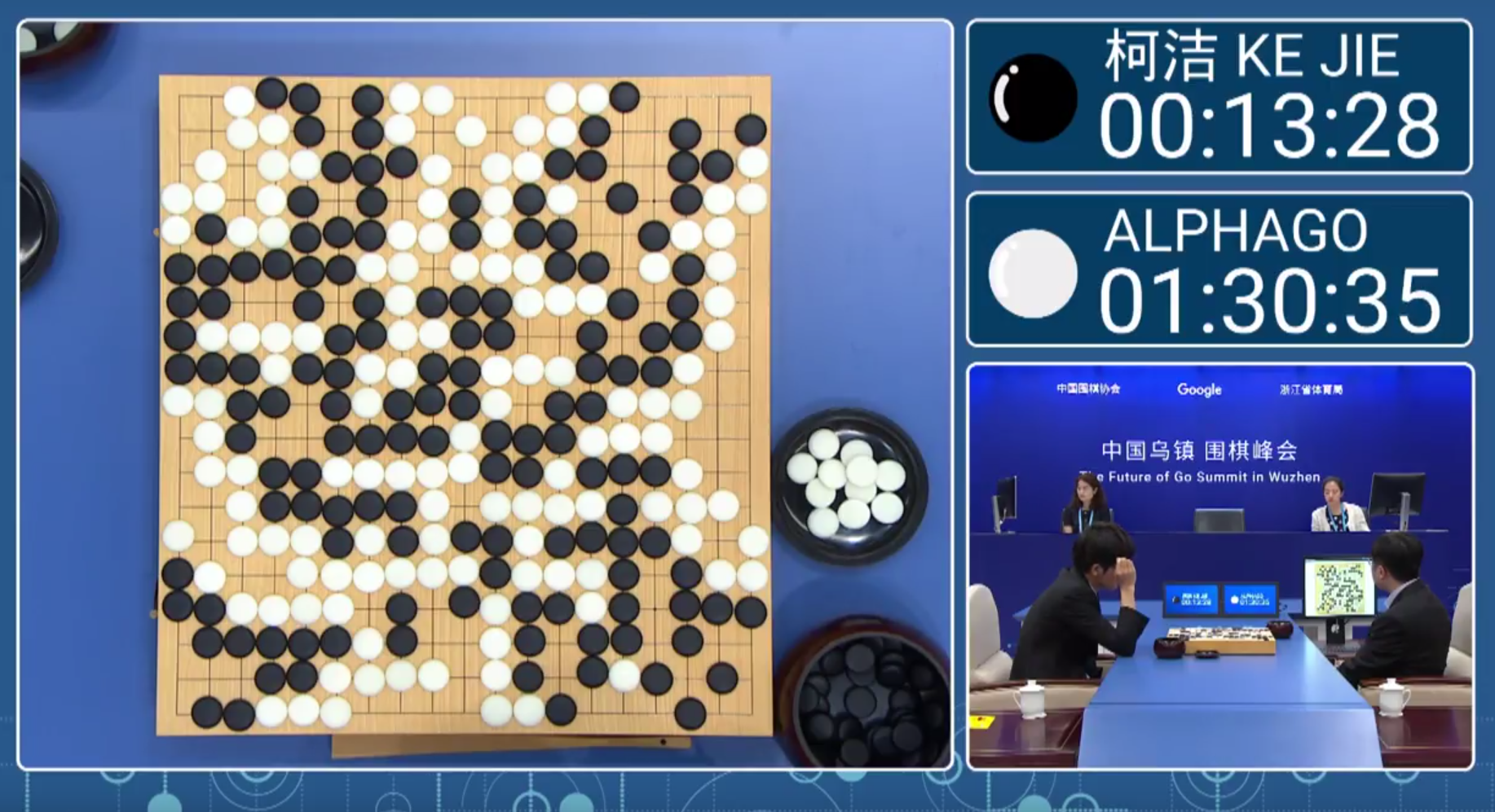
Figure 2: A still frame from the live video feed of the AlphaGo vs. Lee Sedol match.

A related advance was a paper that developed a model that learned to play classic Atari games at a near-human level using as input the raw pixels on the screen (Mnih et al., 2015). This paper was one of the first examples of "Deep RL" - a combination of RL with deep convolutional neural networks from computer vision (more on that later).

Robotics: RL has been used to train robots to perform a wide variety of tasks. For example, RL has been used to train robots to pick and place objects, assemble items, and even fold laundry. These tasks require precise control and adaptation to varying conditions. RL enables robots to learn these tasks through trial and error, improving their ability to operate in dynamic environments. Impressive examples come daily, but one of the more famous is using RL to control autonomous drones to navigate complex environments without human intervention (Zhou et al., 2022). Similarly, RL has been used to create "robotic soccer players" who can learn to play soccer with each other (Stone, Sutton & Kuhlmann, 2005; Kitano et al., 1998).

Figure 3: A youtube video of a swarm RL controlled drones flying through a forest! Scary!

Self-Driving Cars: Companies like Waymo and Tesla use RL to develop self-driving car technology (e.g., Lu et al., 2022). In these cases, one can think of steering a vehicle as a type of dynamic control problem. RL is particularly well suited to these situations. Rewards might be given to keep the car from being in accidents, to stay in the lane, to follow the speed limit, etc... The car can then learn to optimize its behavior to maximize the reward signal.

Human-Computer Interaction: RL is used to optimize user interfaces and, increasingly, in fine-turning the behavior of large language models (LLMs) to generate more human-like text. For example, a technique known as Reinforcement Learning from Human Feedback (RLHF)(?) has been used to train LLMs to generate more human-like text by learning from human feedback on the generated text (Ouyang et al., 2022). Similarly, one futuristic idea is that robots that might live in someone's home could be "taught" to perform different tasks by having the user of the system provide rewards to the robot for doing things correctly. In this case, the human user becomes the "teacher" and the robot the "learner" where rewards and punishments are given by the teacher to shape the behavior of the robot (Amershi et al., 2014).

These are only a few of the many applications of RL. RL is a set of techniques rather than one type of model and so the ideas can be applied to a wide range of problems.

Why is RL interesting in cognitive science?

Reinforcement learning (RL) is highly relevant to cognitive science because it provides a computational framework for understanding how humans and animals learn from their environment through trial and error. Perhaps most importantly, it takes an agentic approach in that it models a primary agent or actor interacting with a dynamic environment. This perspective is sometimes missing from the modeling frameworks we explored in the previous chapter which largely were passive and did not make decisions about how to behave and interact with their environment. For example, simple multi-layer perceptrons are fed inputs selected by the modeler and are given feedback accordingly. In contrast, an RL agent might decide to explore a certain part of their environment and reach a goal. Given that agency, control, and interaction describe the lives of animals and people, RL offers a powerful framework for understanding human cognition.

More specifically, RL algorithms can model how humans learn to make decisions based on rewards and punishments. This type of research has helped cognitive scientists understand how the mechanisms of learning and decision-making work in the brain. RL involves balancing exploration (trying new things) and exploitation (using options known to be rewarding), a topic of immense interest in cognitive science. Furthermore, RL models have been successfully used to account for how people acquire skills, habits, and other patterns of behavior. In recent years, a related field called computational psychiatry(?) has emerged which uses models, many of which borrow from RL concepts, to study disorders like addiction, depression, and obsessive-compulsive disorder (OCD), which involve dysregulation of reward processing and decision-making (Huys, Maia & Frank, 2016). The hope is that insights from these models will inform the development of interventions and therapies that target maladaptive learning patterns.

One of the most compelling examples of RL's relevance to cognitive science is the study of dopamine(?)'s role in reward prediction error. Research has shown that dopamine neurons in the midbrain signal the difference between expected and actual rewards, closely aligning with the reward prediction error signal in RL models (Schultz, Dayan & Montague, 1997; Niv & Schoenbaum, 2008). This discovery has profound implications for understanding learning and decision-making processes, as well as for developing treatments for disorders involving dopaminergic dysfunction.

Besides the theoretical implications, RL algorithms also have useful properties when used as components within larger cognitive models. For example, many problems in cognitive science can abstractly rely on methods like dynamic programming which we discuss below (e.g., Rich & Gureckis, 2018). Similarly, the idea of learning from a reward signal can be used in many types of cognitive models including those based on very complex representations such as neural networks, and even probabilistic programs (e.g., Wang & Lake, 2019). Thus, learning about RL can provide you with a powerful set of tools for developing models of cognition.

RL integrates across Marr's Levels

As mentioned in the introductory reading, research in computational cognitive science often aims analyze behavior at different levels of analysis. In an ideal world, there would eventually be deep integration across the levels (e.g., understanding at the implementational level would align with insights from the computational level). RL is one of a few areas of cognitive science where such synergies exist. At the highest level, the problem of RL is to optimally harvest reward from a potentiall unknown environment. This computational level description highlights the rational basis for behavior and aligns well with ideas in evolution, adaption, etc... As you will read later in this chapter, algorithms developed for RL such as temporal difference (TD) learning are algorithmic solutions to a computational level challenge of optimizing reward. There are many such algorithms which, at a broad level can be seens as using computational algorithms to approximate the computational level problem. However, there is increasing evidence and belief these algorithms are also implemented in the animal brain by the dopaminergic system. Our current understanding suggests this is rare example of a computational theory that seems to connect across levels rather than proceeding independently.

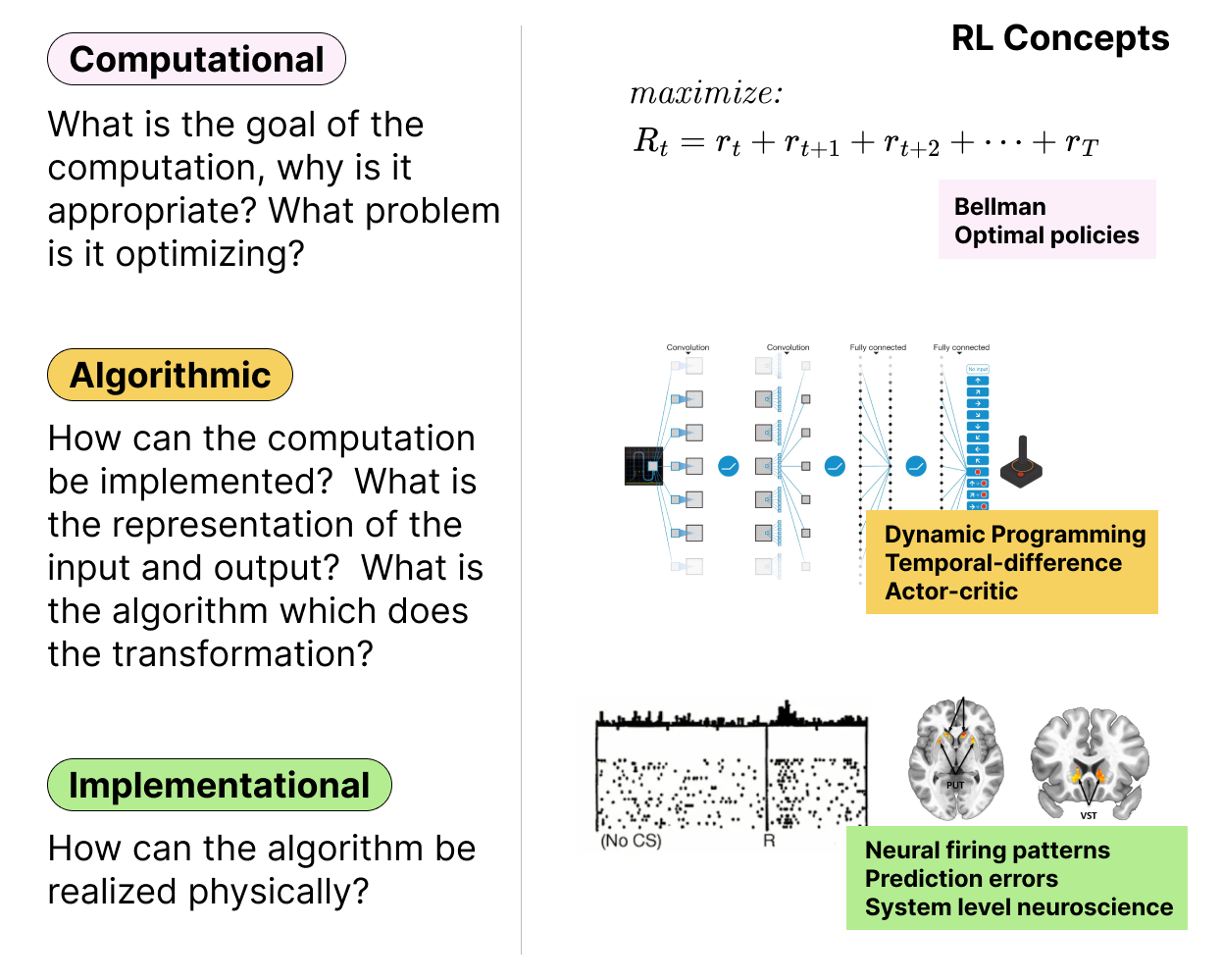
Figure 4: The left panel shows the three levels of analysis proposed by David Marr (computational, algorithmic, and implementational). The right panel shows how aspects of RL theory can be understood at each of these levels. Unlike many areas of cognitive science, research in RL tightly integrates these levels of analysis.

The Problem of RL

As we will see in this chapter, RL is not one algorithm or model but instead a constellation of ideas for how to solve certain types of learning problems. When introducing these algorithms, it helps to start with a clear definition of the problem being solved in RL.

First time with these concetps?

The following section goes through some formal definitions. If you find them confusing or abstract at first, jump ahead to the Gridworld example below and then come back to this section.

At a general level, we can think of RL as a problem involving an agent that interacts with a world or environment. The agent can take actions that change the the environment. The environment responds to the agent's actions by changing its state and providing a reward signal to the agent. The state of the world may be observed by the agent along with the resulting reward signal. The system evolves over time such that the action taken at time $t$ results in rewards $R_{t+1}$ and observation $O_{t+1}$. In the next time step, the agent decides to take another action based on the new reward and observation and so on in a loop. The goal of the agent is to learn how to select actions in such a way that it optimizes the cumulative reward it receives over time. This is illustrated in the following figure:

Figure 5: The basic RL problem.

Let's break this down a bit more. Most RL problems can be described as a Markov Decision Process or MDP. An MDP is a mathematical framework that formalizes the problem of learning from interaction to achieve a goal. Formally, a MDP is defined by a tuple $<S,A,T,R,\gamma >$ where:

• $S$ is the set of states in the environment.
• $A$ is the set of actions the agent can take.
• $T$ is the transition function that specifies the probability of transitioning from one state to another after taking an action.
• $R$ is the reward function that specifies the immediate reward received after taking an action in a state.
• $\gamma$ is the discount factor that determines the importance the solution should place on the future rewards compared to the present.

What do these terms actually mean though? Let's take each one in turn.

States

The state of the environment is a representation of the current situation. It is a summary of all the relevant information that the agent needs to make decisions. For example, in a game of chess, the state might include the positions of all the pieces on the board. In a robotic manipulation task, the state might include the positions of the robot's joints and the objects in the environment.

Understanding what the state is and how it changes is a key part of solving an RL problem. For humans, the state might depend on our limited perceptual abilities. For example, the true state of the environment on a busy street might be very complex but we only attend to a subset of the available information when making decisions about how to cross the street. To distinguish the state from what the agent actually perceives, we introduce the notation of an observation. The observation is the set of features of the state that the agent can actually perceive. The idea is that the environment can be considered to be in on particular state, $s_t$, from a potentially infinite set of states, $S$, defined for any particular problem. For example in chess, $S$ might be all possible gameboard configurations while any particular state $s_t$ is a particular gameboard configuration. The agent might not be able to directly perceive the state $s_t$, but instead observes $o_t$ (an observation of the state). If $o_t=s_t$ then the problem is known as fully observable, in the sense that all aspects of the state are directly available to the agents. If $o_t\ne s_t$ then the problem is partially observable. If the world state is only partially observable then the MDP is a slightly different type of problem called a POMDP (Partially Observable Markov Decision Process), which has its own set of algorithms and challenges (Kaelbling, Littman & Cassandra, 1998).

Actions

An action, $a\in A$, is a decision or move made by the agent from the set of all possible actions. The set $A$ therefore represents the choices that are available to the agent at any given state. The agent selects an action based on its current state and the set of rules for behavior (i.e., policy, see below) it has learned. The action taken by the agent influences the state of the environment and the reward it receives. Not all actions are possible in all states. In addition, actions can be discrete (like a keyboard button press) or continuous (like a joystick movement), depending on the problem. Some RL algorithms only work for discrete action spaces, while others can be adapted for continuous action spaces.

Transition Function

Imagine the agent is in a state $s_t$ and takes an action $a_t$. The next state, $s_t$ is covered by the dynamics of the world. The transition function, $T$, specifies the probability of transitioning from one state to another after taking an action. As a result, it captures the dynamics of the environment and how it changes over time.

The transition function may be deterministic or stochastic. As a result, we typically write the transition function as a probability $P(s_{t+1}|s_t,a_t)$ which is the probability of transitioning to state $s_{t+1}$ given that the agent is in state $s_t$ and takes action $a_t$. The function $T$ is the set of all such probabilities.

States in a MDP have very special property which is that the future state of the environment depends only on the current state and action, not on the history of states and actions that led to the current state. This property is called the Markov property and it simplifies the learning problem and allows for efficient computation of optimal policies. Formally, a state $s_t$ is said to be a Markov state if:

$$P(s_{t+1}|s_t,a_t)=P(s_{t+1}|s_t,a_t,s_{t-1},a_{t-1},\dots )$$

which is to say the probability of the next state depends only on the current state and the action taken and not on the entire history of past states. This is intuitively true for simple games like chess (the probability of the next gameboard configuration depends only on the current gameboard configuration and the move made by the current player). In addition, we typically think of everyday physical systems as following the Markov property because the position of a ball falling from a height depends on its current position and the set of forces currently present and not on the entire history of the ball's motion.

The Markov assumption might seem quite restrictive but in practice is does not strongly limit the types of problems that can be solved with RL. One reason is that the definition of a state, $s_t$ can be quite general. For example, the state of the world might in fact include the state of a memory system inside the agent which can store information about the past. If the state is redefined in this way then the Markov property remains perserved but the history of actions and states taken further in the past can includes the dynamics.

Reward Function

The reward function, $R$, specifies the immediate reward received by the agent after taking an action in a state. The reward is a function of the previous state and the current one, $R(s_t,a_t|s_{t-1})=r$. In RL rewards are almost always assumed to be scalar values that range of $-\mathrm{\infty }$ to $+\mathrm{\infty }$. By convention,larger and positive values indicate relatively good outcomes while smaller and negative values refect bad outcomes.

The reward function provides feedback to the agent about the quality of its actions. The design of a good RL system (i.e., in computer science or engineering) involves finding good ways to design the rewards to encourage the system to do what the designer wants. For example, when designing the robotic drones mentioned above, the designers of the system want to give rewards for good things (staying in the area) while punishments for bad thing (crashing or running into obstacles).

Ultimately, the goal of the agent is to learn a way of behavior (i.e., a "policy") that maximizes the cumulative reward it receives over time. Cummulative rewards are a little different than the immediate reward $r$ given when transitioning from state $s_t$ to $s_{t+1}$ by taking action $a_t$. The cumulative reward, or return, $G_t$, is the sum of all rewards received by the agent from time $t$ onwards:

$$G_t=r_{t+1}+r_{t+2}+r_{t+3}+\dots =\sum _{k=0}^{\mathrm{\infty }}{r}_{t+k+1}$$

RL agents are typically tasked with learning to maximize this quantity. Evolution may have shaped animal behavior in a similar way. Maximizing long term rewards is important because sometimes better outcomes are only available after a series of more costly actions. For example, studying for an exam might locally be a bad experience, but the long term value of getting a good grade might outweight the short, immediate costs. As a result, agents can't simply optimize immediate rewards, but need to consider the long term consequences of their actions.

Discount Factor

In the MDP specification, the final terms is the discount factor, $\gamma$. This reflects an importance given to immediate versus delayed rewards. In the definition of cumulative reward we just defined, we assumed all rewards in time were given equal weight. However, in some cases it can be helpful to specify a weak preference for immediate rewards over delayed ones. This is formalized in a MDP with the discount factor which is typically a value between 0 and 1 that determines the importance the agent places on future rewards compared to immediate rewards.

$$G_t=r_{t+1}+\gamma r_{t+2}+{\gamma }^2{r}_{t+3}+\dots =\sum _{k=0}^{\mathrm{\infty }}{\gamma }^k{r}_{t+k+1}$$

Instead of giving equal weight to all rewards, in this case we "discount" rewards that are further into the future ($t+2,t+3,\dots$) by multiplying them by $\gamma$. Things that are very far into the future are discounted to zero effectively because ${\gamma }^k\to 0$ as $k\to \mathrm{\infty }$ for $\gamma <1.0$.

This is a desirable property because many animals (and people) are known to be a bit myopic in their decision making (Mischel, Shoda & Rodriguez, 1989; Kirby & Herrnstein, 1995; Herrnstein & Prelec, 1991) . For example, people often prefer to receive a small reward now rather than a larger reward later. The discount factor helps to encourage the agent to consider the long-term consequences of its actions and make decisions that maximize the expected cumulative reward over time.

The discount factor also is important for numerical stability. Since the sum of an infinite series of rewards can be infinite, the discount factor helps to ensure that the sum of rewards converges to a finite value. This is important for many RL algorithms that rely on the sum of rewards to estimate the value of states or actions.

One problem definition, maybe specific types

These key components help to defined a MDP and the general RL problem setting in the sense that any particular problem can be described by these components ($<S,A,T,R,\gamma >$). For example, a game like tic-tac-toe can be described by a MDP where the states are the possible board configurations, the actions are the possible moves, the transition function determines how the board changes when a player makes a move, the reward might give a positive value for a win, negative for a loss, and zero for a draw, and the discount factor might be set to 1 because the game is finite and there is no need to discount future rewards. Alternatively in a robotics problem the states might be the possible locations in a building the robot can be, the actions might be the possible movements the robot can make, the transition function might be the physics of the robot's movement, the reward might be a positive value for reaching a goal location and zero otherwise, and the discount factor might be set to 0.9. Each specific problem implies a different defnition or setting of $<S,A,P,R,\gamma >$.

The factors above define the basic structure of the RL problem. However, there are a few other elements worth mentioning that often come in in solutions to MDP. The goal of the agent, faced with any particular MDP or POMDP is to learn a way of behaving that maximizes the long term reward. Often this is accomplished by solve a related problem of estimating the value of particular state or state-action pars. Let's attemp to define these these concepts as well.

Policies

A policy, $\pi$, is a mapping from states to actions that defines the agent's behavior in the environment. The agent's goal is to learn a policy that maps states to actions in a way that maximizes the cumulative reward it receives over time. The policy can be thought of, in the simplest sense, as a lookup table for determining the probability of any action given the current state. For example, a robot might detect it is in a dead end of a hallway. It might consult it's policy for what to do in that case which might be "reverse" or "turn around". We will denote the probability of choose action $a_t$ in state $s_t$ as $\pi (s_t,a_t)$ where $\pi$ refers to all possible values The policy can be deterministic (i.e., it always selects the same action for a given state) or stochastic (i.e., it selects actions probabilistically based on the state). The policy is the agent's strategy for interacting with the environment and achieving its goals. Some policies are good (lead to reliably earning reward) and others are worse, and the goal of learning is to find good policies or even "optimal" policies that maximize the cumulative reward.

Value functions

As we being to think about how to solve RL problem it is helpful to introduce a particular concept called a value function. A value function is not strictly part of an RL problem. In fact, as we will see later, it is possible to learn good behavioral policies without ever referencing the concept of value. However, value functions are a key concept to many RL algorithms. In addition value function relate in a direct way to the concept of utility in economics and psychology.

A value function is a function that estimates the expected cumulative reward that an agent can achieve from a given state or state-action pair. There are two main types of value functions in RL: the state-value (usually denoted as $V(s)$) and the action-value functions (usually denoted as $Q(s,a)$, or called "q-values").

Let's focus on the first one. The value of a state, $V(s)$ is the expected rewards that the agent can expect to receive in the future if it starts in that state and follows a particular policy on all future timesteps. The second part here is important because how good any state is depends directly on what the agent will do in the future. For example, imagine you walk into a bodega and take the action purchase a lottery ticket. If you are handed a winning a lottery ticket, the state of having the winning ticket typically a high value because it leads to future things you could spend money on. The rewards are delayed into the future though -- there's little direct value in holding the ticket. It is what you can do with the ticket in the future that matters. However, imagine you are careless and lose the ticket immediately after winning. This makes clear that the value of a state (i.e., having a winning ticket) also depends on what you do later. If you make good decisions your long term cumulative reward might increase, but if you make bad decisions it might not change much at all (or go down). As a result, the expected reward from any state into the future always depends on the policy.

Given this fact, we can define the value of a given state $V^{\pi }(s)$ under a policy $\pi$ as:

$$\begin{array}{rl}{V}^{\pi }(s)& ={\mathbb{E}}_{\pi }[G_t|s_t=s]\\ & ={\mathbb{E}}^{\pi }\{\sum _{k=0}^{\mathrm{\infty }}{\gamma }^k{r}_{t+k+1}|s_t=s\}\end{array}$$

where ${\mathbb{E}}^{\pi }\{\}$ is the expected value given the agent follows $\pi$ going forward. If we know how much reward we can expect to get from any given state into the future, then we can turn a long term decision making problem (how to make sequences of decisions) into a local one -- we just need to make sure we are always in states with the higher long-term expected value.

The value function is a measure of how good it is to be in a particular state. The action-value function $Q^{\pi }(s,a)$ is the expected return that the agent can achieve from taking action $a$ in state $s$ and then following the policy $\pi$. The only difference is the values ($V^{\pi }(s)$) apply to states themselves whereas state-action values ($Q^{\pi }(s,a)$) are for actions in each state. As we will see later, it is possible to covert between these two representations (the long term value of a state is in fact the average of long term value of each action available in that state weighted by the probability of selecting that action under the current policy, $\pi$). However, we later will discuss ways of learning these quantities directly from experience. In that case sometimes it can be more useful to learn state-action values directly, especially for problems that require the agent to make decision to control their environment.

Gridworlds

To help better understand the concepts of states, actions, rewards, and policies it can help to consider a simplified example. One common example used in RL is the gridworld problem. In this problem, an agent navigates on, typically, a 2d "world" that exists on a grid. The grid is like a maze and at any moment the agent can be in one of the grid cells. There are four actions available in each grid cell location: the agents can choose to move up, down, left, or right.

An example of a grid world is shown here:

Figure 6: Example 2D gridworld problem. The robot is in a world made of grid cells. At each moment they can only occupy one location. Actions (up, down, left, and right) move the robot between the locations. If the agent steps on the green cell they earn a large rewards (+10 points). If they step on the red cell they earn a large penalty (-10 points). The dark grey cell is a barrier and if the agent attempts to move into it they will instead remain in the same location. Each move costs the agent -1 point. Given this decription the goal of the agent is to make as much cumulative reward as possible. This is accomplished by moving efficiently to the goal location (green cell).

Notice the agent is currently at grid cell (0,0). We call this the state of the agnent. The fell set of possible states, $S$, in this problem is all the possible grid cell locations. The trans

The agent receives a reward of -1 for each gridworld environment, moving from one cell to another, with the goal of reaching a specific target cell while avoiding obstacles or hazards.

To summarize, RL problems involve an agent interacting with an environment to learn how to make decisions that maximize cumulative, long-term rewards. The agent's goal is to develop a policy that maps states to actions in a way that maximizes the expected reward over time. The specific class of decision problems that RL addresses are called Markov Decision Processes (MDPs). There are several ways to "solve" a MDP problem and the following sections walk through three foundational approaches which help to introduce the basic ideas underlying RL.

Figure 7: An example of a good and bad solution to this particular gridworld problem. The agent starts in the lower left corner and must reach the green cell. On the right the

The Bellman Equation

Let's first return to our definition of the state-value function, $V^{\pi }(s)$. Early we defined this as the expected cumulative reward that the agent can receive from a given state assuming we then follow the policy $\pi$. The following looks like a lot of math but we are simply making substitutions to quantities we already defined above. For example, first, the value of the state is the long-term return ($G_t$). This is expanded into the exact sum of rewards. Next, we move the $r_{t+1}$ out of the sum (${\gamma }^0=1$) and then add the discounted sum of rewards for $t+2$ onwards. We then explicitly write out the expectation as the sum over the probability of each action available in state $s$ under the policy $\pi$

$$\begin{array}{rl}{V}^{\pi }(s)& ={\mathbb{E}}_{\pi }[G_t|s_t=s]\\ & ={\mathbb{E}}_{\pi }[\sum _{k=0}^{\mathrm{\infty }}{\gamma }^k{r}_{t+k+1}|s_t=s]\\ & ={\mathbb{E}}_{\pi }[r_{t+1}+\gamma \sum _{k=0}^{\mathrm{\infty }}{\gamma }^k{r}_{t+k+2}|s_t=s]\\ & =\sum _a\pi (a|s)\sum _{s^{\prime }}{\mathcal{P}}_{s{s}^{\prime }}^a[{\mathcal{R}}_{s{s}^{\prime }}^a+\gamma {\mathbb{E}}_{\pi }\{\sum _{k=0}^{\mathrm{\infty }}{\gamma }^k{r}_{t+k+2}|s_t=s^{\prime }\}]\\ & =\sum _a\pi (a|s)\sum _{s^{\prime }}{\mathcal{P}}_{s{s}^{\prime }}^a[{\mathcal{R}}_{s{s}^{\prime }}^a+\gamma V^{\pi }(s^{\prime })]\end{array}$$

The final line above is the Bellman equation(?). It is one of the most important equations in RL and understanding it is essential for understanding how RL problems are solved. Let's break down what it means and why it matters.

Why is the Bellman equation important?

The key insight of the Bellman equation is that it expresses the value of a state in terms of the values of its successor states. In other words, the value of where you are right now depends on how good the places you can get to next are. This creates a self-consistency constraint on the values: the value assigned to any state must be consistent with the values of all the states it can transition to. You can't just assign arbitrary values to states -- they have to "agree" with each other according to the structure of the environment and the policy.

This self-consistency is powerful because it means that only certain assignments of values to states are valid. If the values are not self-consistent, they cannot be the true values under the given policy. This dramatically constrains the problem: rather than having to estimate each state's value independently (which would require infinitely long trajectories), we can instead find values that satisfy the Bellman equation simultaneously across all states.

Solving the Bellman equation as a system of equations

Because the Bellman equation defines the value of each state in terms of other states' values, it naturally forms a system of linear equations with $|S|$ unknowns (one for each state). If we know the transition probabilities ${\mathcal{P}}_{s{s}^{\prime }}^a$ and the rewards ${\mathcal{R}}_{s{s}^{\prime }}^a$ -- that is, if we have perfect knowledge of the environment -- we can solve for all the values directly.

To make this concrete, consider a simple gridworld with four states $a,b,c,d$ and a uniform random policy (the agent chooses each of its four actions with probability 0.25). We can "unroll" the Bellman equation for each state. For example, the value of state $a$ might look like:

$$V^{\pi }(a)=0.25[10+V^{\pi }(a)]+0.25[0+V^{\pi }(b)]+0.25[0+V^{\pi }(c)]+0.25[0+V^{\pi }(d)]$$

Here, each term corresponds to one of the four actions: the agent gets an immediate reward (10 or 0 depending on where it ends up) and then lands in a successor state whose value we also need to know. Writing out similar equations for states $b$, $c$, and $d$, and simplifying the notation by replacing $V^{\pi }(a)$ with just $a$, etc., we get a system of equations:

$$\begin{array}{rl}a& =0.25[10+a]+0.25[0+b]+0.25[0+c]+0.25[0+d]\\ b& =0.25[10+a]+0.25[10+b]+0.25[0+c]+0.25[10+d]\\ c& =0.25[10+a]+0.25[0+b]+0.25[0+c]+0.25[10+d]\\ d& =0.25[10+a]+0.25[0+b]+0.25[10+c]+0.25[0+d]\end{array}$$

This is just a system of four equations with four unknowns -- something you could solve with basic linear algebra! The values on the left-hand side also appear on the right-hand side, which is exactly the self-consistency property: each value is defined in terms of the others, and they all have to be solved together. In principle, for any MDP with known dynamics, we can set up and solve a system like this to find the exact values under any policy.

The Bellman equation defines the RL problem

The Bellman equation is important not just as a tool for computation but because it provides the formal foundation for what it means to solve an RL problem. In essence, the goal of RL can be understood as finding values (and ultimately policies) that satisfy the Bellman equation. Many of the algorithms we will study -- dynamic programming, Monte Carlo methods, temporal difference learning -- can be understood as different strategies for finding or approximating solutions to the Bellman equation. Dynamic programming solves it exactly (when the environment is fully known). Monte Carlo and TD methods approximate the solution through experience when the environment is unknown. In this sense, the Bellman equation is the computational-level description of the RL problem, and the various algorithms are different algorithmic-level approaches to satisfying it.

Of course, solving a system of $|S|$ equations directly only works when the state space is small and the environment dynamics are fully known. For most real-world problems -- where the state space is enormous or the dynamics are unknown -- we need approximate methods, which is exactly what the solution methods described below provide.

Overview of solution methods

Now that we have defined the RL problem and the key concepts of states, actions, rewards, policies, value functions, and the Bellman equation, the natural question is: how do we actually solve these problems? There are several foundational approaches, each with different assumptions and trade-offs:

• Dynamic Programming: Dynamic programming methods solve MDPs by computing the optimal value function or policy. These methods are based on the Bellman equations and can be used to find the optimal policy for a given MDP. Although these methods have less applicability to human cognition, they are useful for understanding the theoretical foundations of RL. In some areas, RL is known as "approximate dynamic programming" because it uses computational methods to estimate the solutions one would obtain if dynamic programming could be applied exactly. (Wong et al., 2023)
• Monte Carlo Methods: Monte Carlo methods use random sampling and simulation to estimate the value function or policy of an MDP. These methods are useful when the dynamics of the environment are unknown or when the state space is too large to be explored exhaustively. Aspects of these methods might be relevant to understanding how humans and animals plan.
• Temporal Difference Learning: Temporal difference (TD) learning methods are a class of RL algorithms that combine elements of dynamic programming and Monte Carlo methods. These methods update the value function or policy based on the difference between the predicted and actual rewards. TD learning is a powerful and flexible approach that has been used to model learning in humans and animals.

Over the next few weeks we will dive more deeply into each of these methods, exploring how they work, how they relate to one another, and how they have been used to model human and animal learning and decision-making.

Bibliography

1. Deng, J., Dong, W., Socher, R., Li, L.-J., Li, K., & Fei-Fei, L. (2009). ImageNet: A large-scale hierarchical image database. 2009 IEEE Conference on Computer Vision and Pattern Recognition, 248–255.
2. Barlow, H. B. (1989). Unsupervised learning. Neural Comput., 1(3), 295–311.
3. Lu, Y., Fu, J., Tucker, G., Pan, X., Bronstein, E., Roelofs, R., Sapp, B., White, B., Faust, A., Whiteson, S., Anguelov, D., & Levine, S. (2022). Imitation Is Not Enough: Robustifying Imitation with Reinforcement Learning for Challenging Driving Scenarios.
4. Tesauro, G. (1995). Temporal difference learning and TD-Gammon. Commun. ACM, 38(3), 58–68.
5. Silver, D., Huang, A., Maddison, C. J., Guez, A., Sifre, L., van den Driessche, G., Schrittwieser, J., Antonoglou, I., Panneershelvam, V., Lanctot, M., Dieleman, S., Grewe, D., Nham, J., Kalchbrenner, N., Sutskever, I., Lillicrap, T., Leach, M., Kavukcuoglu, K., Graepel, T., & Hassabis, D. (2016). Mastering the game of Go with deep neural networks and tree search. Nature, 529(7587), 484–489.
6. Mnih, V., Kavukcuoglu, K., Silver, D., Rusu, A. A., Veness, J., Bellemare, M. G., Graves, A., Riedmiller, M., Fidjeland, A. K., Ostrovski, G., Petersen, S., Beattie, C., Sadik, A., Antonoglou, I., King, H., Kumaran, D., Wierstra, D., Legg, S., & Hassabis, D. (2015). Human-level control through deep reinforcement learning. Nature, 518(7540), 529–533.
7. Zhou, X., Wen, X., Wang, Z., Gao, Y., Li, H., Wang, Q., Yang, T., Lu, H., Cao, Y., Xu, C., & Gao, F. (2022). Swarm of micro flying robots in the wild. Sci Robot, 7(66), eabm5954.
8. Stone, P., Sutton, R. S., & Kuhlmann, G. (2005). Reinforcement learning for robocup soccer keepaway. Adapt. Behav.
9. Kitano, H., Tambe, M., Stone, P., Veloso, M., & others. (1998). The RoboCup synthetic agent challenge 97. RoboCup-97: Robot.
10. Ouyang, L., Wu, J., Jiang, X., Almeida, D., Wainwright, C., Mishkin, P., Zhang, C., Agarwal, S., Slama, K., Ray, A., & Others. (2022). Training language models to follow instructions with human feedback. Adv. Neural Inf. Process. Syst., 35, 27730–27744.
11. Amershi, S., Cakmak, M., Knox, W. B., & Kulesza, T. (2014). Power to the people: The role of humans in interactive machine learning. AI Magazine.
12. Huys, Q. J. M., Maia, T. V., & Frank, M. J. (2016). Computational psychiatry as a bridge from neuroscience to clinical applications. Nat. Neurosci., 19(3), 404–413.
13. Schultz, W., Dayan, P., & Montague, P. R. (1997). A neural substrate of prediction and reward. Science, 275(5306), 1593–1599.
14. Niv, Y., & Schoenbaum, G. (2008). Dialogues on prediction errors. Trends Cogn. Sci., 12(7), 265–272.
15. Rich, A. S., & Gureckis, T. M. (2018). Exploratory choice reflects the future value of information. Decisions, 5(3), 177–192.
16. Wang, Z., & Lake, B. M. (2019). Modeling question asking using neural program generation.
17. Kaelbling, L. P., Littman, M. L., & Cassandra, A. R. (1998). Planning and acting in partially observable stochastic domains. Artif. Intell., 101(1), 99–134.
18. Mischel, W., Shoda, Y., & Rodriguez, M. I. (1989). Delay of gratification in children. Science, 244(4907), 933–938.
19. Kirby, K. N., & Herrnstein, R. J. (1995). Preference Reversals Due to Myopic Discounting of Delayed Reward. Psychol. Sci., 6(2), 83–89.
20. Herrnstein, R. J., & Prelec, D. (1991). Melioration: A Theory of Distributed Choice. J. Econ. Perspect., 5(3), 137–156.
21. Wong, L., Grand, G., Lew, A. K., Goodman, N. D., Mansinghka, V. K., Andreas, J., & Tenenbaum, J. B. (2023). From Word Models to World Models: Translating from Natural Language to the Probabilistic Language of Thought.