
Introduction to Jupyter
Contents
3. Introduction to Jupyter#
Note
This chapter authored by Todd M. Gureckis is released under the license for the book. Several of the sections on how to use the Jupyter Interface were developed and shared by Jessica Hamrick as part of a course developed at UC Berkeley.
3.1. Video Lecture#
This video provides an complementary overview of this chapter. There are things mentioned in the chapter not mentioned in the video and vice versa. Together they give an overview of this unit so please read and watch.
3.2. Introduction#
In this lab course you will spend a lot of time analyzing data using computer programs that you partially design yourself. A least part of the toolkit for being a researcher these days involves knowing how to use computers to manipulate and analyze data.
Rather than have everyone in class set up their home computer (which can be difficult across many different home computer types) we will instead use a web-based (or “cloud-based”) solution called JupyterHub. A link to the specific JupyterHub URL for our class this semester is provided in the sidebar of this website.

Fig. 3.1 The Jupyter Project logo.#
JupyterHub lets everyone registered in the class log on to a website and access their own personal set of files. In addition, the instructor can distribute new files to students to work on. Finally, the JupyterHub provides a computing backend which allows you to run several different computer languages. We will focus primarily on Python in this class. Future readings and assignments will introduce the Python programming language to you and also teach you how to use it to analyze data.
However, for now we want to begin by understanding a bit more about Jupyter and the system we will be interacting with.
3.3. Analyzing Data with Computer Scripts#
Doing statistical data analysis using computer scripts written by the researcher is better than point-and-click interfaces such as SPSS that you might be familiar with. If you use a point-and-click interface you have to write down the exact sequence of steps and even take screen-shots of the interface to help someone else perform the same analysis 1. This can lead to bugs and mistakes which hurt the progress of science. In contrast, if your analysis is written in a programming language of some type, the sequence of commands can easily be shared between researchers. Running the sequence of instructions (also referred to as “code”) will allow anyone to repeat the same analysis and check it is correct.
However, writing such code is often kind of limited. Usually computer programs are entered into the computer using a plain text editor (similar to Notepad on the PC or TextEdit on the Mac). This editor cannot display colors (sometimes) and usually also cannot display other types of media like figures, images, tables, movies, interactive animations, and so forth. This makes code somewhat lifeless and also means that any outputs of the code that are media have to be stored separately. For example, if your analysis script outputs a graph, that graph will be saved to a different file and becomes “detached” the code that generated it. This can make it hard to keep track of outputs and can lead to errors.
The “notebook” interface is an approach to a programming and data analysis which combines programming/analysis code with text, images, figure, animations, and other multimedia in the same document (see Figure 3.2). The idea for computational notebooks has been around for a long time (e.g., Mathematica is a commercial product that has long provided a notebook interface for data analysis and programming). However, Jupyter is now one of the leading tools that scientists, including psychological/cognitive scientists, use to analyze their data and write code.
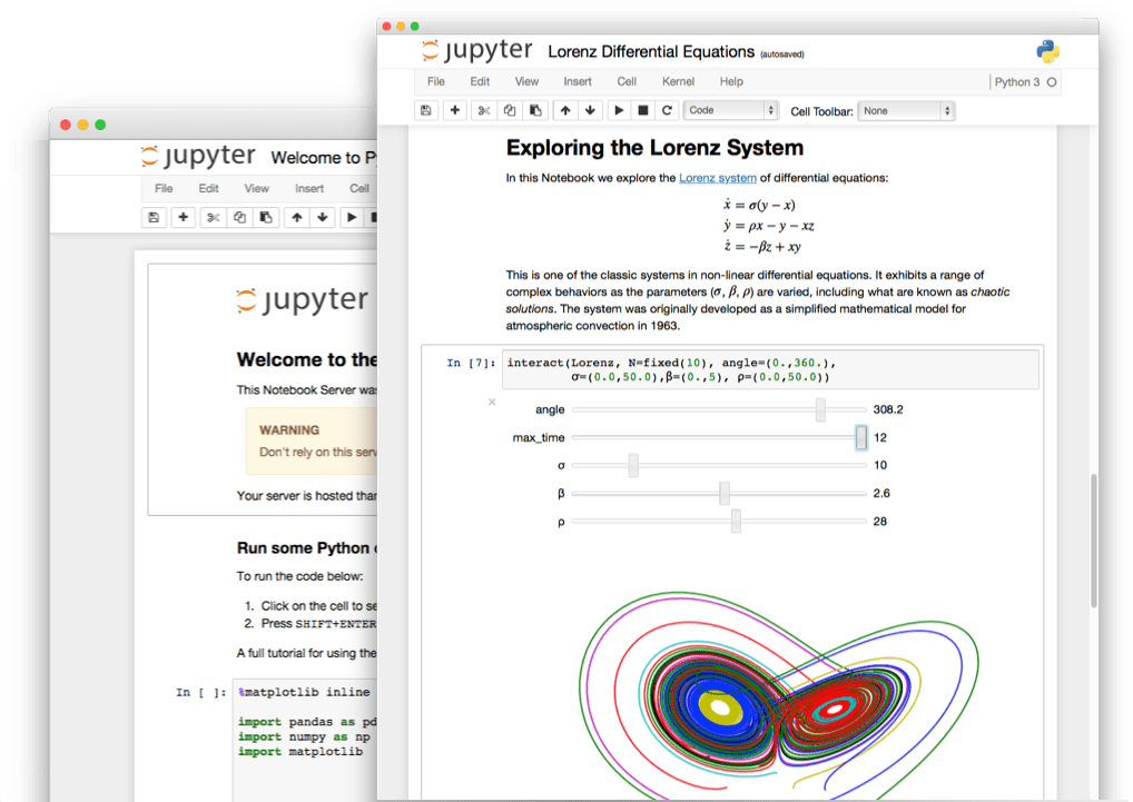
Fig. 3.2 A screenshot of a Jupyter Notebook. Notice how the document combines text, pictures and analysis code.#
There are several reasons for the popularity of Jupyter:
Jupyter is open source and free. This means it is not owned by any one person or company. Scientists and other programmers devote their time to improving Jupyter. The code is readable by anyone which means it is easier to catch bugs.
Jupyter works with several different programming languages including R, Python, Matlab and others which are popular for data analysis.
Jupyter runs in a standard webbrowser. This means you can use Jupyter often on any computing device you like including low-cost laptops like Chromebooks/Netbooks or even a tablet like an iPad.
Jupyter has many extensions which provide interactive widgets, animations, beautiful graphics, etc…
Jupyter is fun! Once you get the hang of the notebook concept then it makes develping and debugging code a pretty fun experience.
Many companies use Jupyter internally and are looking to hire people with this skill.
External Reading
If you are registered for the course please read this article before continuing this chapter [Per18].
3.4. Every chapter of the class website/textbook is a Notebook#
One sort of interesting feature of this class is that more or less everything uses Jupyter notebooks. This includes the class webpage and each chapter of the online textbook. In fact the document you are reading was first entered in as a Jupyter notebook. Using the Jupyterbook these notebooks were converted to a webpage. However, you can easily open the notebook the was used to write this chapter and check out the code and run it yourself 2.
There are two key ways to do this. First, in the top right of this webpage you should see a little menu option that looks like this:

Fig. 3.3 The JupyterBook menus for our online textbook.#
The button with the little arrow pointing down will let you download the current chapter either as a .ipynb (i.e., a Jupyter notebook) or as a PDF. If you download the notebook to your computer you can easily upload it to a running Jupyter/JupyterHub instance. For example, if you login to the class JupyterHub you can upload the .ipynb, open it, and then begin interacting with is such as executing the cells, editing them, and interacting with widgets and other interactive animations.
Even easier, if you are registered for the course (this will not work for people viewing these pages on line) you can launch any of the chapters of the textbook on your own Jupyter instance by clicking on the buttons shown here:

Fig. 3.4 The JupyterBook menu to launch the current book notebook on your own personal Jupyterhub (registered students only).#
Others viewing these pages can choose the Google Colab option.
In addition, for most of the computer-generated graphs and tables in the book you can view the code used to create the figure. Just look for something that looks like this:
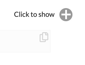
Fig. 3.5 Click this button to reveal the python code used to generate the figure, table, graph or other output.#
3.5. The “notebook” and “kernel” concepts#
The key to Jupyter is the concept of a computational notebook. A computational notebook is a document-based approach to structuring data analysis and programming. A notebook appears and acts similar to other programs you are familiar with like Excel or Google Sheets (spreadsheets) or Word or Google Docs (word processor). These programs provide ways for you to enter information into documents and to save those file, send them to others, copy-paste, text, alter the formatting, etc…
We will primarily use the “classic” Jupyter Notebook interface which consists of a single document which you interact with not unlike a word processor. There is a newer interface called JupyterLab which looks more like Matlab or RStudio’s interface allowing multiple windows and views of the running code. The traditional notebook interface is prefered here primarily because it simple and faciliates reading along.
A computational notebook typically is made up of a set of elements called “cells” that group little bits of information together. A notebook document (usually ending with the .ipynb extension on the file name) is a list of cells arranged from the top of the document to the bottom. Cells can contain several types of information including code, text, images and so forth. You develop your project by creating new cells, entering information, reordering cells, and saving the results.
The key element which makes a notebook “computational” is that it can be linked to a computing engine known as a “kernel” which can run on the same computer or another computer using the Internet. The kernel is separate from the notebook and can for instance be stopped and started independently from the program displaying the notebook itself. The magic happens when a cell is “executed.” This sounds scary but refers simply to making the code in the cell “go”. When this happens the code from the cell that was executed is sent to the computational kernel and this kernel will run the sequence of commands contained within the cell. Any results such as figures or printouts from the results of that code running will be sent to the notebook from the kernel and will be inserted beneath the cell which was just executed. A diagram of the basic conceptual idea is shown in Figure 3.6.
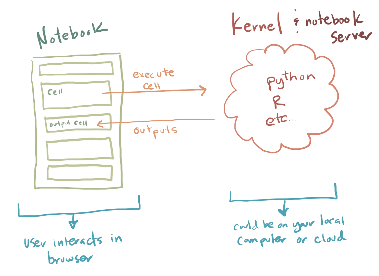
Fig. 3.6 The flow between the notebook and the kernel. Cells when they are executed are sent to the computational kernel which is an independent piece of software which can be started and stopped independently from the notebook.#
3.6. Caution: The Notebook State and Kernel State are not the Same!#
One somewhat confusing aspect of Jupyter for beginners is that the notebook is simply a way to organize information and the order of information in a notebook has nothing to do with the order in which code has been executed on the server.
Instead, each time you execute a cell, the commands from that cell are sent to the kernel, run, and then returned. Usually it make sense to organize your code so that multiple cells are arranged in order from the top of the document to the bottom. You would then execute the first cell, then the second cell, and so forth.
However, and this is really important, you don’t have to execute the cells in order. You can execute the third cell before the second or first cell if you want. This just means that the code in the third cell would be sent to the kernel first and then the other cells would be sent. This means that the order of the cells in the notebook document are really just for presentation, and it is up to you to “run/execute” the cells in whatever order you want.
This is mostly helpful because when you are doing and analysis you might want to go back up to the top and change something and then continue where you left off. To do that you could scroll back to a earlier cell, change it, then execute it and then go back down to the beginning of the script.
However, things can get confusing. If you delete a cell it doesn’t mean the code was “undone”. The kernel doesn’t know anything about any edits you make to the notebook interface. All it does is receive code when you send it via the “execute cell” command and then it waits. This can mean that the “state” or current status of the kernel can at times be different from what your cells or notebook look like. One easy option to deal with this is that if things get too far out of wack you can simply restart the kernel. This will erase it’s current state and set it back to a fresh start. However, then you need to re-execute all of the cells in your notebook to get back to where you were.
The best analogy is like telling your friend how to cook a meal for you over the phone. You have the instructions in front of you (your notebook) and you tell your friend (the kernel) what to do. If you read the instructions out of order your friend can’t tell the difference. They just know each step you told them to do and follow it. It is up to you to direct the instructions so they arrive to your friend (the kernel) in the right order. And of course if things get confused you can just tell your friend to start over from stratch and begin again.
At first this can be confusing but eventually you get the hang of it. It is one source of bugs/errors in Jupyter programming though and some people don’t like using Jupyter for that reason. In our case the upsides overweight this awkwardness.
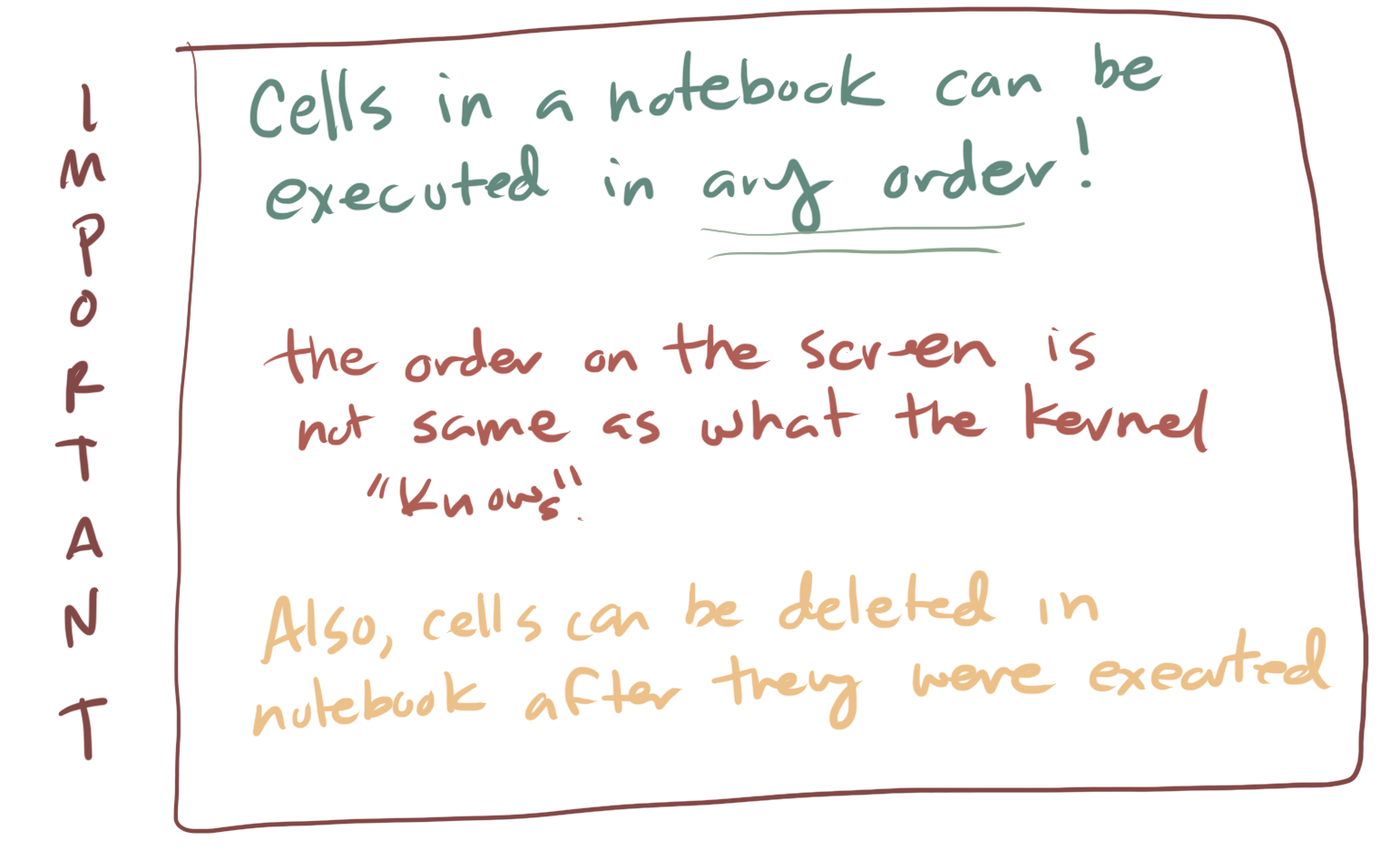
Fig. 3.7 Important facts that the notebook interface and the order things are sent to the kernel is up to you. Also cells can be deleted or added in the notebook interface and the kernel doesn’t know this.#
3.7. Overview of the Jupyter Notebook#
In the following section we will go over the basics of the Jupyter interface. While you can easily read this file on the web as a reminder it can be helpful to actually open this file in Jupyter so you can follow along and see the interface as it will actually appear. Refer to the earlier section for several methods for opening this file in a Jupyter instance.
First, as described, notebooks are made up of a series of cells. For example, the text you are reading is in what is called a “Markdown cell”. The following cell is a “code cell”:
# this is a code cell
You can tell what the type of a cell is by selecting the cell, and looking at the toolbar at the top of the page. For example, try clicking on this cell. You should see the cell type menu displaying “Markdown”, like this:
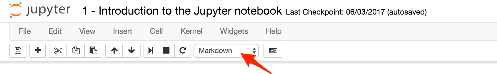
Fig. 3.8 The menu option that lets you control which “type” a cell is.#
3.8. Command mode and edit mode#
In the notebook, there are two modes: edit mode and command mode. By default the notebook begins in command mode. In order to edit a cell, you need to be in edit mode.
Command Mode
When you are in command mode, you can press enter to switch to edit mode. The outline of the cell you currently have selected will turn green, and a cursor will appear.
Edit Mode
When you are in edit mode, you can press escape to switch to command mode. The outline of the cell you currently have selected will turn gray, and the cursor will disappear.
3.8.1. Markdown cells#
For example, a markdown cell might look like this in command mode (Note: the following few cells are not actually cells – they are images and just look like cells! This is for demonstration purposes only.)

Fig. 3.9 A Markdown cell in command mode.#
Then, when you press enter, it will change to edit mode:

Fig. 3.10 A Markdown cell in edit mode.#
Now, when we press escape, it will change back to command mode:

Fig. 3.11 A Markdown cell based in command mode, but not it is not rendered into HTML.#
However, you’ll notice that the cell no longer looks like it did originally. This is because IPython will only render the markdown when you tell it to. To do this, we need to “run” the cell by pressing Ctrl-Enter, and then it will go back to looking like it did originally:
Fig. 3.12 A Markdown cell “executed” to that it renders into HTML.#
Note
You will frequently use Markdown cells to give answers to homework questions so it is useful to learn a little bit of the Markdown syntax.
3.8.2. Code cells#
For code cells, it is pretty much the same thing. This is what a code cell looks like in command mode (again, the next few cells LOOK like cells, but are just images):

Fig. 3.13 A code cell in command mode.#
If we press enter, it will change to edit mode:

Fig. 3.14 A code cell in edit mode.#
And pressing escape will also go back to command mode:
Fig. 3.15 A code cell in command mode again after pressing escape.#
If we were to press Ctrl-Enter like we did for the markdown cell, this would actually run the code in the code cell:

Fig. 3.16 Pressing ctrl-enter executes the cell by sending the code to the kernel associated with the notebook.#
3.9. Executing cells#
Code cells can contain any valid Python code in them. When you run the cell, the code is executed and any output is displayed.
Note
You can execute cells with Ctrl-Enter (which will keep the cell selected), or Shift-Enter (which will select the next cell).
Try running the following cell and see what it prints out:
print("Printing cumulative sum from 1-10:")
total = 0
for i in range(1, 11):
    total += i
    print("Sum of 1 to " + str(i) + " is: " + str(total))
print("Done printing numbers.")
You’ll notice that the output beneath the cell corresponds to the print statements in the code. Here is another example, which only prints out the final sum:
total = 0
for i in range(1, 11):
    total += i
print(total)
Another way to print something out is to have that thing be the last line in the cell. For example, we could rewrite our example above to be:
total = 0
for i in range(1, 11):
    total += i
total
However, this will not work unless the thing to be displayed is on the last line. For example, if we wanted to print the total sum and then a message after that, this will not do what we want (it will only print “Done computing total.”, and not the total sum itself).
total = 0
for i in range(1, 11):
    total += i
total
print("Done computing total.")
If you are accustomed to Python 2, note that the parentheses are obligatory for the print function in Python 3.
3.10. The IPython kernel#
When you first start a notebook, you are also starting what is called a kernel. This is a special program that runs in the background and executes code (by default, this is Python, but it could be other languages too, like R!). Whenever you run a code cell, you are telling the kernel to execute the code that is in the cell, and to print the output (if any).
Just like if you were typing code at the Python interpreter, you need to make sure your variables are declared before you can use them. What will happen when you run the following cell? Try it and see:
a
The issue is that the variable a does not exist. Modify the cell above so that a is declared first (for example, you could set the value of a to 1 – or pick whatever value you want). Once you have modified the above cell, you should be able to run the following cell (if you haven’t modified the above cell, you’ll get the same error!):
print("The value of 'a' is: " + str(a))
Running the above cell should work, because a has now been declared. To see what variables have been declared, you can use the %whos command:
%whos
If you ran the summing examples from the previous section, you’ll notice that total and i are listed under the %whos command. That is because when we ran the code for those examples, they also modified the kernel state.
(Note that commands beginning with a percent (%) or double percent (%%) are special IPython commands called magics. They will only work in IPython.)
3.10.1. Restarting the kernel#
It is generally a good idea to periodically restart the kernel and start fresh, because you may be using some variables that you declared at some point, but at a later point deleted that declaration.
Warning
Your code should always be able to work if you run every cell in the notebook, in order, starting from a new kernel.
To test that your code can do this, first restart the kernel by clicking the restart button:
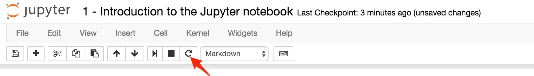
Fig. 3.17 The button to restart the kernel#
Then, run all cells in the notebook in order by choosing Cell\(\rightarrow\)Run All from the menu above.
Keyboard Shortcuts
There are many keyboard shortcuts for the notebook. To see a full list of these, go to Help\(\rightarrow\)Keyboard Shortcuts.
User Interface Tour
To learn a little more about what things are what in the IPython Notebook, check out the user interface tour, which you can access by going to Help\(\rightarrow\)User Interface Tour.
3.11. Markdown and LaTeX Cheatsheet#
As mentioned above, Markdown is a special way of writing text in order to specify formatting, like whether text should be bold, italicized, etc. In a homework you will get some practice with this. However, you can always come back and use the following website as a reference: https://help.github.com/articles/markdown-basics
Hint #1: after editing the Markdown, you will need to run the cell so that the formatting appears.
Hint #2: try selecting this cell so you can see what the Markdown looks like when you’re editing it. Remember to run the cell again to see what it looks like when it is formatted.
Markdown is a useful tool in Jupyter for making things look nice but you don’t have to be a Markdown expert to succeed at this class.
3.12. Additional Resources#
This chapter gives you a basic introduction to the Jupyter Notebook system we will be using more or less daily in this class. It is something you will get more familiar with through experience. However, if you want additional resources here are some useful guides and videos introducing Jupyter:
3.13. References#
- Per18
J.M." Perkel. Why jupyter is data scientists' computational notebook of choice. Nature, 563:145–146, 2018.
- 1
Note that some point and click analysis programs do allow some types of scripting. However, the primary way people use and are taught these tools is through the graphical interface (in fact this is primarily why these programs are popular!)
- 2
The book chapters have some additional formatting for the web that you might not see in a regular notebook. However most of this just looks like more complex Markdown.